A coding-focused introduction to Deep Learning using PyTorch, starting from the very basics and going all the way up to advanced topics like Generative Adverserial Networks
Requirements
Basic knowledge of Python
Basic linear algebra (vectors, matrices etc.)
Description
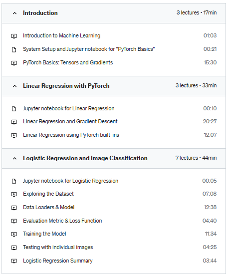
“PyTorch: Zero to GANs” is an online course and series of tutorials on building deep learning models with PyTorch, an open source neural networks library. Here are the concepts covered in this course:
PyTorch Basics: Tensors & Gradients
Linear Regression & Gradient Descent
Classification using Logistic Regression
Feedforward Neural Networks & Training on GPUs (this post)
Coming soon.. (CNNs, RNNs, transfer learning, GANs etc.)
This course will be updated on a weekly basis with new material.
Who this course is for:
Students and developers curious about data science
Data scientists and machine learning engineers curious about PyTorch
No experience required, the course start from cero
Description
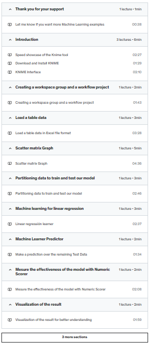
In last couple of years, machine learning has become a fundamental tool for decision-making in the corporate world, as well as widely used in different areas, ranging from business to the purest science, allowing the computer to perform the most difficult tasks finding patterns and correlations between variables that allow through inferential statistics to make predictions based on data, which allows creating competitive advantages in various fields, taking advantage of the inputs of historical information of the company or business to find patterns and correlations that allow us to identify possible future outcomes. Under the supervised learning paradigm we will apply the concept of linear regression to project, through the equation of the line, the possible result values in relation to predictor variables and dependent variables, in which Machine Learning is able to identify the weights of importance for each one of the participating variables, its relationship with the variable of interest to be predicted and even determine if any system variable can be discarded, in order to create a model with a high level of statistical reliability that contributes to the decision-making process management, finally one of the objectives of the course is to also understand the importance of data visualization to achieve a greater understanding of the results of the model and thus identify how far or close to the actual results selected to evaluate the model we are
Who this course is for:
decision makers, data analist, students, and people interested in learn to use machine learning
Use Python for Machine Learning to classify breast cancer as either Malignant or Benign.
Implement Machine Learning Algorithms
Exploratory Data Analysis
Learn to use Pandas for Data Analysis
Learn to use NumPy for Numerical Data
Learn to use Matplotlib for Python Plotting
Use Plotly for interactive dynamic visualizations
Learn to use Seaborn for Python Graphical Representation
Logistic Regression
Random Forest and Decision Trees
Requirements
Basics of Python
Some high school mathematics level.
Some programming experience
Description
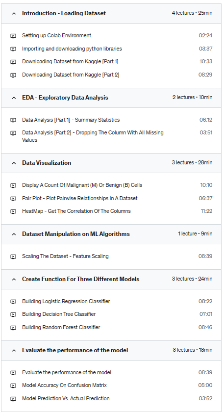
Here you will learn to build three models that are Logistic regression model, the Decision Tree model, and Random Forest Classifier model using Scikit-learn to classify breast cancer as either Malignant or Benign.
We will use the Breast Cancer Wisconsin (Diagnostic) Data Set from Kaggle.
Prerequisite
You should be familiar with the Python Programming language and you should have a theoretical understanding of the three algorithms that is Logistic regression model, Decision Tree model, and Random Forest Classifier model.
Learn Step-By-Step
In this course you will be taught through these steps:
Section 1: Loading Dataset
Introduction and Import Libraries
Download Dataset directly from Kaggle
2nd Way To Load Data To Colab
Section 2: EDA – Exploratory Data Analysis
Checking The Total Number Of Rows And Columns
Checking The Columns And Their Corresponding Data Types (Along With Finding Whether They Contain Null Values Or Not)
2nd Way To Check For Null Values
Dropping The Column With All Missing Values
Checking Datatypes
Section 3: Visualization
Display A Count Of Malignant (M) Or Benign (B) Cells
Visualizing The Counts Of Both Cells
Perform LabelEncoding – Encode The ‘diagnosis’ Column Or Categorical Data Values
Pair Plot – Plot Pairwise Relationships In A Dataset
Get The Correlation Of The Columns -> How One Column Can Influence The Other Visualizing The Correlation
Section 4: Dataset Manipulation on ML Algorithms
Split the data into Independent and Dependent sets to perform Feature Scaling
Scaling The Dataset – Feature Scaling
Section 5: Create Function For Three Different Models
Building Logistic Regression Classifier
Building Decision Tree Classifier
Building Random Forest Classifier
Section 6: Evaluate the performance of the model
Printing Accuracy Of Each Model On The Training Dataset
Model Accuracy On Confusion Matrix
2nd Way To Get Metrics
Prediction
Conclusion
By the end of this project, you will be able to build three classifiers to classify cancerous and noncancerous patients. You will also be able to set up and work with the Google colab environment. Additionally, you will also be able to clean and prepare data for analysis.
Who this course is for:
Interested in the field of Machine Learning? Then this course is for you!
This course had been designed to be your guide to learning how to use the power of Python to analyze data, create some good beautiful visualization for better understanding and use some powerful machine learning algorithms.
This course will also give you a hands-on walk through step-by-step into the world of machine learning and how amazing it is to make prediction on some serious real-life problems. This course will not only help you develop new skills and improve your understanding but also grow confidence in you.
It is undeniably, machine learning and artificial intelligence have become immensely notorious over the past few years. Also, at the moment, big data is gaining notoriety in the tech industry where machine learning is amazingly powerful for delivering predictions or forecasting recommendations, relied on the huge amount of data.
What are Machine Learning Algorithms?
Being a subset of Artificial Intelligence, Machine Learning is the technique that trains computers/systems to work independently, without being programmed explicitly.
And, during this process of training and learning, various algorithms come into the picture, that helps such systems in order to train themselves in a superior way with time, are referred as Machine Learning Algorithms.
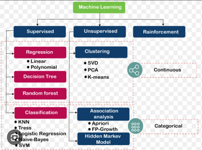
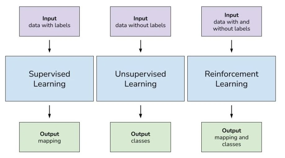
Machine learning algorithms work on the concept of three ubiquitous learning models: supervised learning, unsupervised learning, and reinforcement learning. These are essentially the types of machine learning;
Supervised learning is deployed in cases where a label data is available for specific datasets and identifies patterns within values labels assigned to data points.
Unsupervised learning is implemented in cases where the difficulty is to determine implicit connections in a given unlabeled dataset.
Reinforcement learning selects an action, relied on each data point and after that learn how good the action was.
(Related blog: Fundamentals to Reinforcement Learning)
Machine Learning Algorithm
In the intense dynamic time, several machine learning algorithms have been developed in order to solve real-world problems; they are extremely automated and self-correcting as embracing the potential of improving over time while exploiting growing amounts of data and demanding minimal human intervention.
Let’s learn about some of the fascinating machine learning algorithms;
Decision Tree
The decision tree is the decision supporting tool that practices a tree-like graph or model of decisions along with their feasible outcomes, like the chance-event outcome, resource costs and implementation.
Being a supervised learning algorithm, decision trees are the best choice for classifying both categorical and continuous dependent variables. In this algorithm, the population is split into two or more homogeneous datasets, relying on the most significant characteristics or independent variables.
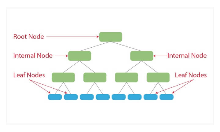
Over the graphical representation of the decision tree, the internal node highlights a test on the attribute, each individual branch denotes the outcome of the test, and leaf node signifies a specific class label, therefore the decision is made after computing all the attributes.
Fundamentally, decision trees are of two types;
Classification Trees– Accounted as the default kind of decision trees, classification trees are adapted to distinct the dataset into various classes on the basis of the response variable, and preferred when the response variable is categorical in nature.
Regression Trees– In opposite to the classification tree, regression trees are chosen when the response or target variable is continuous or numerical in nature and adapted in predictive based problems.
Naive Bayes Classifier
A Naive Bayes classifier believes that the appearance of a selective feature in a class is irrelevant to the appearance of any other feature. It considers all the properties independent while calculating the probability of a particular outcome, even if each feature are related to each other.
The model involves two types of probabilities
Probability of each class, and
Conditional Probability for each class, given each x value.
Both the probabilities can be measured directly from training data, once calculated, the probability model can be deployed for making predictions for new data via Bayes Theorem.
Some of the real-world cases of naive Bayes classifiers are to label an email as spam or not, to categorize a new article in technology, politics or sports group, to identify a text stating positive or negative emotions, and in face and voice recognition software.
Ordinary Least Square Regression
Under statistics computation, Least Square is the method to perform linear regression. In order to establish the connection between a dependent variable and an independent variable, the ordinary least squares method is like- draw a straight line, later for each data point, calculate the vertical distance amidst the point and the line and summed these up.
The fitted line would be the one where the sum of distances is as small as possible. Least squares are referring to the sort of errors metric that are minimized.
Linear Regression
Linear Regression describes the impact on the dependent variable while the independent variable gets altered, as a consequence an independent variable is known as the explanatory variable whereas the dependent variable is named as the factor of interest.
It shows the connection amid an independent and a dependent variable and deals with prediction/estimations in continuous values. E.g. it can be used for risk assessment in the insurance domain, to identify the number of applications for multiple ages users.
The linear regression can be described in terms of a best fit relationship among the input variable (x) and output variable (y) through identifying the specific weights for the input variables, named as coefficients (B), that is
y= B0 + B1*x
Logistic Regression
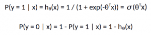
Logistic regression is a powerful statistical tool of modelling a binomial outcome with one or more explanatory variables. It computes the association amid the categorical dependent variable and one or more independent variables through measuring probabilities by a logistic function (or cumulative logistics distribution).
The Logistic Regression Algorithm works for discrete values, it is well suitable for binary classification where if an event occurs successfully, it is classified as 1, and 0, if not. Therefore, the probability of occurring of a specific event is estimated in the basis of provided predictor variables.
It has the real world applications as;
Credit scoring
Estimating success rates of marketing campaigns
Anticipating the revenues generated by a certain product or service.
In politics, whether a particular candidate wins or loses the election.
Support Vector Machines
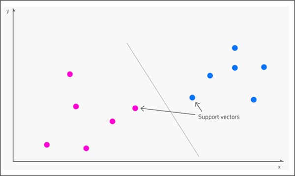
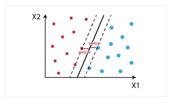
In SVM, a hyperplane (a line that divides the input variable space) is selected to separate appropriately the data points across input variables space by their respective class either 0 or 1.
Basically, the SVM algorithm determines the coefficients that yield in the suitable separation of the various classes through the hyperplane, where the distance amid the hyperplane and the closest data points is referred to as the margin. However, the optimal hyperplane, that can depart the two classes, is the line that holds the largest margin.
Only such points are applicable in determining the hyperplane and the construction of the classifier and are termed as the support vectors as they support or define the hyperplane.
More specifically, SVM renders appropriate classification for classification problems upon the training data, and extra efficiency for accurate classification of the future and also doesn’t overfit the data.
SVM is greatly used for stock market forecasting, for instance, one can use it to check the relative performance of the one stocks when compared to the other stocks under the same market. Thereby, with the help of the relative comparison of stocks, one can manage investment and make decisions depending upon the classifications made by SVM algorithm.
Clustering Algorithms
Being an unsupervised learning problem, clustering approach is used as a data analysis technique for identifying informative data patterns, such as groups of customers based on their behavior or locations. Clustering descibes a class of problem and a class of methods, take a look at Clustering Methods and Applications.
Clustering Algorithms refer to the group task of clustering, i.e. grouping an assemblage of objects in such a way that each object is more identical to each other under the same group (cluster) in comparison to those in separate groups.
There are various kinds of clustering algorithms that use similarity or distance measures amid examples in the feature space to find out dense regions of observations. Therefore, it is a good attempt to scale data previously for using clustering algorithms. However, each clustering algorithm is different, some of them are connectivity-based algorithms, dimensionality reduction, neural networks, probabilistic, etc.
Gradient Boosting & AdaBoost
Boosting algorithms are used while dealing with massive quantities of data for making a prediction with great accuracy. It is an ensemble learning algorithm that integrates the predictive potential of diversified base estimators in order to enhance robustness, i.e. it blends the various vulnerable and mediocre predictors for developing strong predictor/estimator.
In simple terms, Boosting is the learning algorithm that makes an active classifier/predictor from a weak or average classifier. This process is achieved through creating a model from training data, and then constructing another second model in order to correct the errors from the first model. Also, until the training set is precisely predicted, models are added or until the maximum number of models are joined.
These algorithms usually fit well in data science competitions like Kaggle, Hackathons, etc. As treated most preferred ML algorithms, these can be used with Python and R programming for obtaining accurate outcomes.
AdaBoost was the first competitive boosting algorithm that was constructed for binary classification. It can be considered as the initial step for learning and understanding boosting. Most of the modern boosting methods are constructed over AdaBoost, preferably on stochastic gradient boosting machines.
The video below explains the AdaBoost which is just the simple twist on decision trees and random forests.
Principal Component Analysis
Dimensionality reduction algorithms are among the most important algorithms in machine learning that can be used when a data has multiple dimensions.
Consider a dataset that has “n” dimension, for instance a data professionlist is working on financial data that has the attributes as a credit score, personal details, personnel salary, etc. Now, in order to understand the important labels for building a required model, he/she can use dimensionality reduction method, and PCA is the appropriate algorithm for reducing dimensions.
PCA is a statistical approach that deploys an orthogonal transformation for reforming an array of observations of likely correlated variables into a set of observations of linearly uncorrelated variables, is known as principal components.
Using PCA, one can decrease the quantity of dimensions while retaining the important labels of the model. Since PCA is heavily relied on the number of dimensions, each PCA is perpendicular to the other and their dot product is zero.
Its applications include analysing data for smooth learning, and visualization. Since all the components of PCA have a very high variance, it is not an appropriate approach for noisy data.
Deep Learning Algorithms
Deep learning algorithms heavily rely on the nervous system of a human and are generally designed on the neural networks that use plentiful computational resources. All these algorithms use different types of neural networks to perform particular tasks.
They train computers by learning from examples and industries such as healthcare, eCommerce, entertainment, and advertising commonly use deep learning algorithms.
Since, the deep learning algorithms signify self-learning representations, they basically coin ton ANNs that reflect the way a human brain functions and computes information. While the training process starts, algorithms intakes unknown components as the input data for extracting out features, group objects, and find out useful and hidden data patterns.
These algorithms make use of several algorithms where no one single network is considered perfect and some algorithms are perfect fitted to perform specific tasks. However, in order to choose the correct ones, one should have a strong understanding of all primary algorithms
Some popular deep learning algorithms are Convolutional Neural Network (CNN), Recurrent Neural Networks (RNN), Long Short-Term Memory Networks (LSTM), etc.
Conclusion
From the above discussion, it can be concluded that Machine learning algorithms are programs/ models that learn from data and improve from experience regardless of the intervention of human being.
Google’s self-driving cars and robots get a lot of press, but the company’s real future is in machine learning, the technology that enables computers to get smarter and more personal. – Eric Schmidt (Google Chairman)
Some popular examples, where ML algorithms are being deployed, are Netflix’s algorithms that recommend movies based on the movies (or movie genre) we have watched in past, or Amazon’s algorithms that suggest an item, based on review or purchase history.
All machine learning fields—Supervised, Unsupervised, Semi-supervised, and Reinforcement learning, use several algorithms for different types of tasks like prediction, classification, regression, etc. Each machine learning algorithm handles one specific problem, and this way beginners can dive into one of these to figure out solutions, one at a time.
Here is a compilation of the top machine learning algorithms that are frequently used in all machine learning fields.
Now, you can practice ML algorithms here.
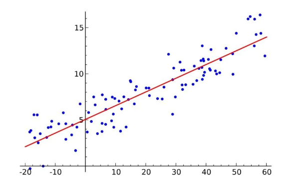
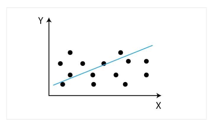
Linear regression
Forming relationships between two variables is almost the starting point of a model, and linear regression in machine learning achieves that. The relationship between the dependent and independent variables is established by aligning them on a regression line. Then, the objective is to find the best fit line that explains the relationship between both variables.
The linear regression line is represented by a mathematical equation by,
y = mx + c
Where y is the dependent variable, x is the independent variable, m is the slope, and c is the intercept.
Logistic regression
Now, when the dependent variable is dichotomous (binary), logistic regression is used to estimate the discrete values (unlike linear regression that handles continuous values) within a set of independent variables.
This algorithm is used in predictive analysis where probability of an event occurrence is predicted based on logit function, which is why it is also called ‘logit regression’.
Mathematically, it is represented by,
y = e^(b0 + b1*x) / (1 + e^(b0 + b1*x))
Where x is the input value, y is the predicted output, b0 is the bias, and b1 is the coefficient for x.
Artificial neural networks
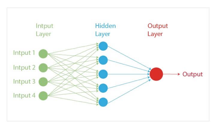
ANNs are used in most of the recent AGI-related models that use self-supervised learning. This algorithm tries to mimic the human brain by copying the behaviour and connections of the neurons. The structure of ANNs has three or more layers that are interconnected for processing input data.
These are used in various smart appliances as well as automation devices like automatic cars, smart speakers and lights, and much more.
Convolutional neural networks (CNNs), one of the most used neural networks in recent developments, are a type of ANNs. These are mostly computer vision-based networks where the first layer is the input layer, the layers in between are the hidden layers that do that computing, and the third layer is the output layer.
Gradient descent
An optimisation algorithm for minimising cost function by updating parameters of the machine learning model. It is used inside various machine learning algorithms and is most commonly used in deep learning. It is used in various fields like robotics, computer games, mechanical engineering, and more.
There are three types of gradient descent algorithms:
Batch gradient descent: Processes all the training data for each iteration of gradient descent. If the dataset is large, this method is too expensive.
Stochastic gradient descent: This processes one training example per iteration, resulting in parameters getting updated every single time.
Mini batch gradient descent: The fastest gradient descent that processes large amounts of iterations in small batches, matching similar iterations.
Decision trees
A supervised learning algorithm used for visualisation of a map of possible results for a series of decisions. Basically, it splits the dataset into two or more homogeneous for comparison of possible outcomes and then makes decisions based on advantages and probabilities.
It is like making a pros and cons list, and making decisions based on anticipations and potentiality of different options but, in machine learning, it is based on a mathematical construct.
Naive Bayes Algorithm
Bayesian probability is a type of probability concept where instead of frequency of a phenomenon, probability is interpreted by quantification of a personal belief or knowledge representing a reasonable expectation. The Naive Bayes is used for classification problems, and it assumes that features in the algorithm are independent of each other and are not impacted by changes in each other.
For example, the weight and size of a table can change and maybe interrelated but do not change the fundamental fact that it is a table. This simplistic algorithm is capable of handling large datasets and making predictions in real-time.
Bayes’ theorem is given by,
P (X|Y) = (P (Y|X) x P (X)) /P (Y)
Where P(X) is the probability of X being true, P(X/Y) is the conditional probability where X is true when Y is true as well.
KNN Algorithm
This supervised machine learning algorithm classifies all new cases based on old cases stored that are segregated into different classes based on their similarity scores. K Nearest Neighbours (KNN) is used for both regression and classification problems.
K refers to the number of nearby points considered during segregation and classification of a set of known groups. The algorithm does classification by a majority vote of the neighbouring K points.
Major use cases and real-life applications of the algorithm can be found in recommendation systems of OTT platforms like Amazon and Netflix, and also facial recognition systems.
K-Means
For clustering tasks, K-means is an unsupervised machine learning algorithm based on distance. The algorithm classifies datasets into K clusters where within one set, the data points remain homogenous, but not in different clusters.
This algorithm is used in clustering Facebook users who have common interests based on their likes and dislikes, and also segmentation of similar eCommerce products.
Random forest algorithm
Another supervised learning algorithm, Random trees is a collection of multiple decision trees that are built on different samples during training. It builds on the accuracy of decision trees by mapping decisions from different trees onto a single tree known as a CART model (Classification and Regression Trees).
This helps in increasing accuracy when in a dataset, a large chunk of data is missing. The final prediction is based on the prediction result which is voted the highest. This algorithm is mostly used in eCommerce recommendation engines and financial models.
Support Vector Machines
SVMs are supervised machine learning algorithms that plot individual data into a number of dimensional spaces, based on the number of features. Classification is performed by determining the hyper-plane that distincts two sets of support vectors.
Simply, SVMs are for representing coordinates of individual observations. These are popularly used in machine learning applications like facial expression classification, speech recognition, and image detection.
015 key limitations of machine learning algorithms
02When is a machine learning application not the best choice?
03With all its limitations, is ML worth using?
Over the past few years, artificial intelligence (AI) and machine learning (ML) developers have made AI and ML think more like humans, performing complex tasks and making decisions based on deep analysis. Robots performing various jobs for humans are no longer the plot of science fiction films, but the reality of today. However, despite the progress data scientist teams have made in this field, there are still several limitations of machine learning algorithms.
The number of AI consulting agencies has skyrocketed over the past few years, accompanied by a 100% increase in AI-related jobs between 2015 and 2018. This boom has fueled the growth of ML in all kinds of industries.
While ML is very useful for many projects, sometimes it’s not the best solution. In some cases, ML implementation is not necessary, does not make sense, and can even cause more problems than it solves. This article discusses instances where ML is not an appropriate solution.
Want to know more about tech trends?
5 key limitations of machine learning algorithms
ML has profoundly impacted the world. We are slowly evolving towards a philosophy that Yuval Noah Harari calls “dataism”, which means that people trust data and algorithms more than their personal beliefs.
If you think this definitely couldn’t happen to you, consider taking a vacation in an unfamiliar country. Let’s say you are in Zanzibar for the first time. To reach your destination, you follow the GPS instructions rather than reading a map yourself. In some instances, people have plunged full speed into swamps or lakes because they followed a navigation device’s instructions and never once looked at a map.
ML offers an innovative approach to project development that requires processing a large amount of data. But what key issues should you consider before you choose ML as a tool to develop for your startup or business? Before implementing this powerful technology, you must be aware of its potential limitations and pitfalls. ML issues that may arise can be classified into five main categories, which we highlight below.
Ethical concerns
There are, of course, many advantages to trusting algorithms. Humanity has benefited from relying on computer algorithms to automate processes, analyze large amounts of data, and make complex decisions. However, trusting algorithms has its drawbacks. Algorithms can be subject to bias at any level of development. And since algorithms are developed and trained by humans, it’s nearly impossible to eliminate bias.
Many ethical questions still remain unanswered. For example, who is to blame if something goes wrong? Let’s take the most obvious example — self-driving cars. Who should be held accountable in the event of a traffic accident? The driver, the car manufacturer, or the developer of the software?
One thing is clear — ML cannot make difficult ethical or moral decisions on its own. In the not too distant future, we will have to create a framework to solve ethical concerns about ML technology.
Deterministic problems
ML is a powerful technology well suited for many domains, including weather forecasting and climate and atmospheric research. ML models can be used to help calibrate and correct sensors that allow you to adjust the operation of sensors that measure environmental indicators like temperature, pressure, and humidity.
Models can be programmed, for example, to simulate weather and emissions into the atmosphere to forecast pollution. Depending on the amount of data and the complexity of the model, this can be computationally intensive and take up to a month.
Can humans use ML for weather forecasting? Maybe. Experts can use data from satellites and weather stations along with a rudimentary forecasting algorithm. They can provide the necessary data like air pressure in a specific area, the humidity level in the air, wind speed, etcetera, to train a neural network to predict tomorrow’s weather.
However, neural networks do not understand the physics of a weather system, nor do not understand its laws. For example, ML can make predictions, but the calculations of such intermediate fields as density can have negative values that are impossible under the laws of physics. AI does not recognize cause-and-effect relationships. The neural network finds a connection between input and output data but cannot explain the reason they are connected.
Lack of Data
Neural networks are complex architectures and require enormous amounts of training data to produce viable results. As the size of a neural network’s architecture grows, so does its data requirement. In such cases, some may decide to reuse the data, but this will never bring good results.
Another problem is related to the lack of quality data. This is not the same as simply not having data. Let’s say your neural network requires more data, and you give it a sufficient quantity, but you give it poor quality data. This can significantly reduce the model’s accuracy.
For example, suppose the data used to train an algorithm to detect breast cancer uses mammograms primarily from white women. In that case, the model trained on this dataset might be biased in a way that produces inaccurate predictions when it reads mammograms of Black women. Black women are already 42% more likely to die from breast cancer due to many factors, and poorly trained cancer-detection algorithms will only widen that gap.
Lack of interpretability
One significant problem with deep learning algorithms is interpretability. Let’s say you work for a financial firm, and you need to build a model to detect fraudulent transactions. In this case, your model should be able to justify how it classifies transactions. A deep learning algorithm may have good accuracy and responsiveness for this task but may not validate its solutions.
Or maybe you work for an AI consulting firm. You want to offer your services to a client that uses only traditional statistical methods. AI models can be powerless if they cannot be interpreted, and the process of human interpretation involves nuances that go far beyond technical skill. If you can’t convince your client that you understand how an algorithm comes to a decision, how likely is it that they will trust you and your experience?
It is paramount that ML methods achieve interpretability if they are to be applied in practice.
Lack of reproducibility
Lack of reproducibility in ML is a complex and growing issue exacerbated by a lack of code transparency and model testing methodologies. Research labs develop new models that can be quickly deployed in real-world applications. However, even if the models are developed to take into account the latest research advances, they may not work in real cases.
Reproducibility can help different industries and professionals implement the same model and discover solutions to problems faster. Lack of reproducibility can affect safety, reliability, and the detection of bias.
When is a machine learning application not the best choice?
Nine times out of ten ML should not be applied with no labeled data and personal experience. Almost always labeled data is essential for deep learning models. Data labeling is the process of marking up already “clean” data and organizing it for machine learning. If you do not have enough high-quality labeled data, the use of ML is not recommended.
Another example of when to avoid AI is in designing mission-critical security systems because ML requires more complex data than other technologies.
The more data needs to be processed, the greater the complexity and vulnerability. This includes aircraft flight controls, nuclear power plant controls, and so on.
With all its limitations, is ML worth using?
It cannot be denied that AI has opened up many promising opportunities for humanity. However, it’s also led some to philosophize that machine learning algorithms can solve all of humanity’s problems.
Machine learning systems work best when applied to a task that a human would otherwise do. It can do well if it isn’t asked to be creative, intuitive, or use common sense.
Algorithms learn well from explicit data, but it doesn’t understand the world and how it works the way we humans do. For example, an ML system can be taught what a cup looks like, but it doesn’t understand that there is coffee in it.
People feel these limitations, like common sense and intuition, when they interact with AI. For example, chatbots and voice assistants often fail when asked reasonable questions that involve intuition. Autonomous systems have blind spots and fail to detect potentially critical stimuli that a person would immediately notice.
The power of machine learning helps people do their jobs more efficiently and live better lives, but it cannot replace them because it cannot adequately perform many tasks. ML offers certain advantages but also some challenges.
At Postindustria, we are skilled in overcoming the limitations and have extensive experience in ML development. We are ready to take on your project. Leave us your contact details and we will reach out to discuss your solution.
Types of Learning Styles for Machine Learning Algorithms
Before we begin discussing specific algorithms, however, we need a basic understanding of the different learning styles often seen in machine learning algorithms. These learning styles are supervised, unsupervised, and semi-supervised learning.
Types of Machine Learning and Differences Between Learning Styles
Supervised Learning
Supervised learning is a technique where a task is accomplished by providing training (input and output) patterns to the systems. Supervised learning in machine learning maps an input to its outputs based on sample input-output pairs. This type of learning infers a function from labeled and organized training data that consists of sets of training examples.
Datasets used for training with supervised learning are labeled with X and Y-axis variables and usually consist of metadata rather than image inputs. A popular example of a supervised learning dataset is the University of California Irvine Iris Dataset where the predicted attribute is the class of Iris (a type of flower) and the inputs are different variables depicting Iris classes (petal width and length, sepal width and length).
Supervised learning models are prepared through a training process where the model is required to make predictions and corrects itself when those predictions are incorrect. This guess-and-check type process continues until the model achieves a predetermined level of accuracy using the given training data.
Algorithms used for supervised learning are logistic regression and back propagation neural networks. Machine learning problems regarding supervised learning often involve classification and regression.
Unsupervised Learning
Unsupervised learning for machine learning does not require the creator to “supervise” the model during training. Unsupervised learning allows the model to discover patterns independently of a well-organized and labeled dataset. This is why unlabeled datasets are used often for unsupervised learning to generate machine learning models.
Unsupervised learning leaves algorithms to find structure in the inputs without the use of predefined variable names or labels.
While supervised learning models are given the inputs and left to predict the outputs, unsupervised learning models predict both the inputs and the outputs. This is done by detecting prominent patterns between inputs and associating those with potential outputs.
Algorithms specific to unsupervised machine learning models include K-means and the Apriori algorithm. Popular machine learning problems that can be solved using unsupervised learning involve clustering, dimensionality reduction, and association rule learning.
Semi-supervised Learning
Semi-supervised learning is the middle ground between unsupervised and supervised learning. Semi-supervised learning usually requires a combination of a small amount of labeled data and a comparatively large amount of unlabeled data for training its machine learning models.
As with supervised learning, example machine learning problems that can be solved with semi-supervised learning include classification and regressions. Semi-supervised learning is useful for image classification purposes but is still debated on whether it is the most efficient for that purpose.
Regression Algorithms for Machine Learning
Algorithms allow for sectors of machine learning like unsupervised, supervised, and semi-supervised learning to be productive.
Regression algorithms can be used for supervised and semi-supervised learning, and specifically deal with modeling the relationship between variables. It is refined iteratively using a measure of error in the predictions made by the model at hand. Regression is both a type of machine learning problem and algorithm.
For our intents and purposes, we are discussing regression as it relates to being a type of error-based machine learning algorithm. Popular regression algorithms include a handful, but the most relevant to us in this article are linear, logistic, and ordinary least squares regression.
Simple Linear Regression for Machine Learning
Regression is a method of modeling a target value based on independent predictors. This makes regression a good method for modeling a target value based on independent predictor variables.
Linear regression for machine learning algorithms Simple linear regression is a relatively easy concept for a machine learning model algorithm in part due to its simplicity. The number of independent variables is 1, and there is a linear relationship between the independent and dependent X and Y variables. The line of best fit models given points in a dataset with the most accuracy. The line is then modeled with a linear equation where y = A0 + A1(x) → or y = mx + b.
Error Function
The error function (also known as “cost function”) is used to provide the “best” line of best fit for our respective data points. The search problem is converted into a minimization problem where the error between the predicted value and actual value is the least. In other words, the error function captures the error between the predictions made by a model versus the actual values in a training dataset.
Linear regression as an algorithm aims to find the best fitting values for A0 and A1 which is a two-part process that can be better understood by learning about cost function and gradient descent.
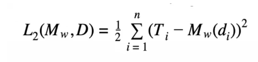
Sum of Squared Errors Error Function
The above mathematical representation is the formal definition of the sum of squared errors error function. Keep in mind that M is the complete machine learning model at hand, instead of a variable that represents a single value.
The training set given is composed of n training instances, each of which have d descriptive features and T single-target feature. Mw (d) is the prediction made by the candidate model at hand for any given training instance containing di descriptive features. The machine learning aspect of this function can be seen where the candidate model Mw is defined by the weight vector w.
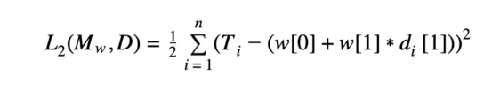
If we take, for example, a scenario where each instance is described with a single descriptive feature (meaning each independent data point maps to a singular dependent data point as the descriptive feature), the equation can expand to something like the following:
Expanded Error Function
The weights can change, there is a corresponding sum of squared errors value for every possible combination of weights (weights are also known as model parameters). The key to using simple linear regression models is determining the optimal values for the weights using the equation.
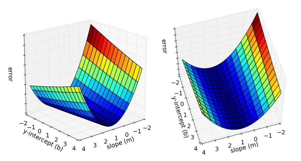
Error Surfaces to Find Optimal Values
Error Surfaces to Determine Optimal Values The sum of squared errors function can be used to measure how well any combination of weights fits the respective instances in a dataset. Instead of using a brute-force search to find the best combination, we can use associated error surfaces to calculate the optimal combination of weights.
The error surfaces for any machine learning simple regression problem are convex (shaped like a bowl). We want to use the error surfaces to find a unique set of optimal weights with the lowest sum of squared errors (finding the global minimum). Finding the global minimum uses a process known as least squares optimization.
Least Squares Optimization
As mentioned earlier, we can predict that the error surface of our algorithm will produce a convex shape, thus possessing a global minimum. The distinctive shape of the error surfaces can be attributed to it being defined mostly by the linearity of the model, rather than the properties of the data. This means the partial derivatives of the error surface with respect to weights (w[0] and w[1]) are equal to 0 because they measure the slope of the error surface at the points w[0] and w[1].
The bottom of the error surface is not curved and does not have any slope, due to the convex shape, which is why the partial derivatives of the error surface are 0 at that point. We can infer that because of the aforementioned properties, that point is the global minimum of the error surface and are exactly the points we would need to calculate the most efficient weights to use for machine learning.
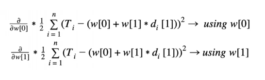
So how do we calculate the global minimum? By combining the equation discussed earlier for simple linear regression with partial derivatives, we can define the global minimum on the error surface as:
Global Minimum on the Error Surface
Multivariable Linear Regression with Gradient Descent
Multivariable linear regression with gradient descent can be used to train a best-fit model for a given training set and is one of the most common approaches to doing so within error-based machine learning.
It is still used only for supervised and semi-supervised learning because a dataset is required. While the simple linear regression section above dealt with a single descriptive feature, multivariable linear regression models can handle more than one descriptive features (and are thus, multivariable).
A random example of a machine learning model where this type of algorithm would be useful is for predicting the price of a house in a neighborhood where variables like land size, crime rate, and miles from schooling are integral to the fluctuating price of the house.
Multivariable Linear Regression Mathematical Representation
We can actually take our simple linear regression representation from earlier in the article and extend it to include an array of variables rather than just one.
variables extended simple linear regression representation
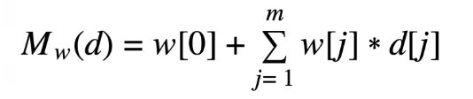
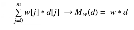
In this instance, d is the array of m descriptive features. Thus, d[1]…d[m] represents all descriptive features, while w[1]…w[m] are m+1 weights. We can then simplify the above expansion by using a nonexistent descriptive feature, d[0], which is equal to 1. This then produces:
expanded simple linear regression representation
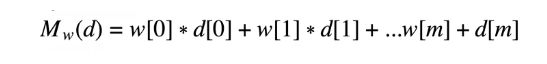
We can easily spot the summation process in this equation, so we can replace it with sigma, and reduce the sum of all descriptive features to just Mw(d) =w*d.
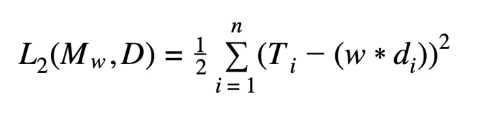
What this means, in essence, is that w*d is the sum of the products of the arrays’ w and d corresponding elements. The loss function calculated earlier (L2) can be altered to reflect the new regression equation which takes into account multi variability.
Summation Process Replaced
What this means, in essence, is that w*d is the sum of the products of the arrays’ w and d corresponding elements. The loss function calculated earlier (L2) can be altered to reflect the new regression equation which takes into account multi variability.
Multivariable Model Accounting for Dot Product
Here, w*d is representative of the dot product of the vectors w and d, as deduced earlier. The above multivariable model allows us to include more than one descriptive feature in a concise way. An example of the equation using real-life variables (referring to our house-price example) would be: price = w[0] +w[1] * landSize + w[2] *crimeRate
Gradient Descent as a Concept
Finding the best-fit set of weights for machine learning with multivariable regression is done using a process called gradient descent. The previous global minimum approach is not as effective for multivariable regression as it is for simple linear regression because the number of instances in the training set and number of weights make the equation not computationally feasible.
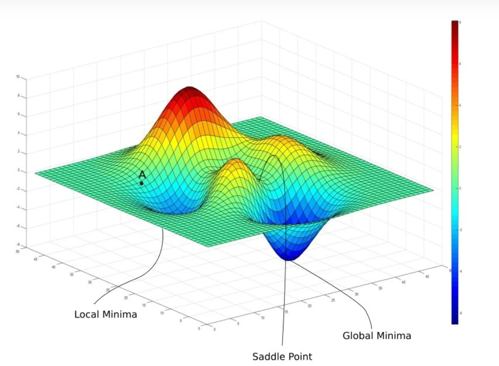
We can still, however, use error surfaces as part of the gradient descent process to calculate the global minimum (which is different from simple linear regression). Instead of visualizing a simple, bowl-shaped error surface, imagine a non-convex error surface where there are peaks and valleys – similar to a mountainous landscape:
Set of weights for machine learning with a gradient descent method.
Gradient descent begins by selecting a random point within the space of weight. Our algorithm can only use local information from around this point because the rest of the space is unknown. Using the slope of the error surface at that location, the randomly selected weights can then be adjusted little by little in the direction of the error surface gradient to move to a new position on the error surface.
The adjustments are made in the direction of the error surface gradient, allowing for each new point to be slightly closer to the overall global minimum, until the global minimum is reached (where the slope is 0). The saddle point in the above image is the random point we start with. We then go to the local minimum and keep iterating the process until the global minimum is achieved.
Gradient Descent as an Algorithm (Batch Gradient Descent)
The gradient descent algorithm for training multivariable linear regression models requires a set of training instances (referred to as D), as well as a learning rate (α) for controlling the rate at which the algorithm converges, a convergence criterion that indicates when to stop the algorithm iterations, and lastly, an error delta function that determines the direction in which to adjust the randomized weight for coming closer to the global minimum.
Taking into consideration more than one variable changes the previous sum of squared errors for each training instance to:
Multivariable Sum of Squared Errors
Just as a reminder, D in this case refers to the set of training instances and w[j] (discussed later) is the randomly selected beginning weight.
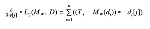
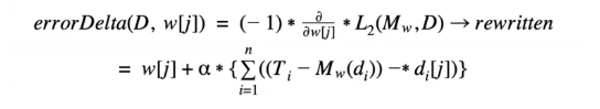
Error Delta Function for Multivariable Linear Regression
For each calculated gradient using the above equation for machine learning algorithms, we want to move in the opposite direction for the purpose of returning a lower value on the error surface. The error delta function calculates the delta value that determines the direction and the magnitude of the adjustments made to each weight.
The delta value is determined by the gradient of the error surface at the latest position in the space of weight. Therefore, our error delta function (whose purpose is to calculate the direction to move in for a given weight), is:
The above is the weight update rule for multivariable linear regression with gradient descent, where tiis the expected target feature for i training instance and relates to w (the weight vector), di [j] (j^th descriptive feature corresponding to the i^th instance of training), and (the constant learning rate). The error delta function is the lower equation starting with the sigma sign (in curly brackets) within the greater weight update rule.
Error Delta Function
The above is the weight update rule for multivariable linear regression with gradient descent, where ti is the expected target feature for i training instance and relates to w (the weight vector), di [j] (j descriptive feature corresponding to the i instance of training), and (the constant learning rate). The error delta function is the lower equation starting with the sigma sign (in curly brackets) within the greater weight update rule.
Understanding the Weight Update Rule
Understanding the weight update rule for machine learning algorithms starts with understanding how it changes weights based on the error calculations by predictions made in the current candidate model.
If the errors show that predictions made by the model at hand are too high, then the weights should be decreased while di [j] is positive and increased while negative.
If the errors show that predictions made by the model at hand are too low, then the weights should be increased while di [j] is positive and increased while negative.
This process in its entirety is also known as “batch gradient descent” because one adjustment is made to each weight for each iteration, so the weights are changed in “batches.”
Logistic Regression
Logistic regression is useful when the dependent variable is “binary” in nature. This means logistic regression is usually associated with examining the association of independent variables with one dichotomous dependent variable. Meanwhile, linear regression is used for when the dependent variable is continuous, and the nature of the line of regression is linear.
A random example of how logistic regression has been used as an algorithm for machine learning is modeling how new words enter a language over time or how the amount of people using a product changes its buying patterns over time.
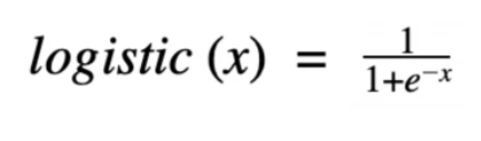
Logistic Regression Function
For logistic regression models, the output of the basic linear regression model is outputted using the logistic function. The logistic function is a threshold function that is continuous and differentiable.
Logistic Function
For reference, the above equation represents e as Euler’s number (2.71828), the base of the natural logarithms, and x as the input value.
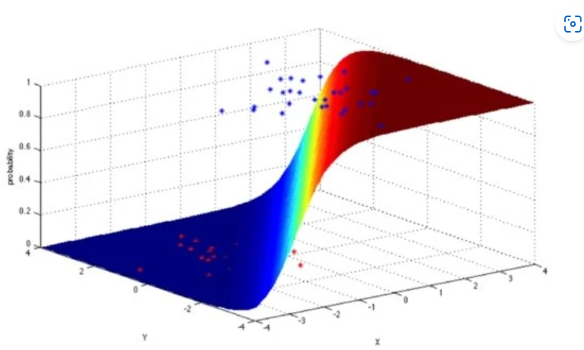
Instead of the regression function being the dot product of the weights and descriptive features like in linear and multivariable regression functions, the logistic function passes the dot products of weights and descriptive feature values through it. The decision surface that results from the above equation once values are substituted is quite different from the error surfaces we saw earlier for multivariable and linear regression.
Decision Surface for Logistic Regression
The decision surface for logistic regression is not to be confused with the error surfaces discussed earlier – they are two separate ideas. The decision surface shows the value of the logistic equation for every possible input value. Logistic regression usually has a gentle transition from faulty target predictions to good target predictions.
This is a benefit for using logistic regression, since the correct and incorrect prediction accuracies are not as “black and white” as they are for simple linear and multivariable regression. Logistic regression models can also be interpreted as probabilities of the occurrence of a target level (through the use of the logistic function).
A subset of artificial intelligence, machine learning is a class of methods for automatically creating models from data. Using the relationships derived from the training dataset, these models are then able to make predictions on unseen data. Machine learning algorithms are the engine for machine learning because they turn a dataset into a model. Different types of algorithms learn differently (supervised learning, unsupervised learning, reinforcement learning) and perform different functions (classification, regression, natural language processing, and so on).
The algorithm you select depends on the type of machine learning problem you’re solving, available computing resources, and the nature of the dataset (eg: labeled vs. unlabeled). Generally, machine learning algorithms are used for classification or prediction problems. When a model is “fit” on a dataset, it learns from the data by recognizing patterns in the data.
Remember that machine learning algorithms are different machine learning models, although these terms are often used interchangeably. A model in machine learning is the output of a machine learning algorithm that has been fit on a dataset. The model represents what the algorithm has learned from the data—the rules, numbers, and other algorithm-specific data structures required to make predictions.
ML algorithms can be described using math and pseudocode (a representation of code that can be understood by a layman). Algorithmic pseudocode is a plain language description of the steps in an algorithm.
In the real world, machine learning algorithms are used on massive datasets to perform a range of prediction tasks, such as powering recommendation engines and performing spam and fraud detection, risk assessments, image and text classification, natural language processing, sentiment analysis, and so much more.
Is machine learning the right career for you? Find out if you’re eligible for Springboard’s Machine Learning Career Track.
What are the 3 Types of Machine Learning Algorithms?
Machine learning algorithms can be programmed to learn from data in different ways. The most common types of machine learning algorithms make use of supervised learning, unsupervised learning, and reinforcement learning.
1. Supervised learning
Supervised learning algorithms learn by example. The programmer provides the machine learning algorithm with a known dataset that includes desired inputs and outputs (such as input images and their corresponding labels), and the algorithm determines how to arrive at the desired output (known as “ground truth”) by identifying patterns in the training data.
The algorithm learns from these observations, makes predictions on test data, and is corrected by the programmer. In the end, the programmer picks the model or function that best describes the training data and makes the best estimation of output. Supervised learning is useful for image classification, regression, and forecasting.
2. Unsupervised learning
Unsupervised learningalgorithms make predictions from untagged data, where there is no ground truth or known output. Unsupervised learning algorithms can discover hidden patterns or data groupings to analyze and cluster unlabeled datasets—making them the ideal solution for exploratory data analysis. The algorithm classifies, labels, and/or groups the data points without any human intervention.
While unsupervised learning can perform more complex data mining tasks than supervised learning algorithms, they can be more unpredictable, potentially adding categories and labels based on its interpretation of the training data. This type of algorithm whose logic can’t be explained in plain language is known as a “black box.” Unsupervised learning is useful for customer segmentation, anomaly detection in network traffic, and content recommendations.
3. Reinforcement learning
Reinforcement learning algorithms follow a regimented learning process of trial-and-error. The algorithm is provided with a set of actions, parameters, and values—similar to the types of constraints players face in a game. The algorithm then tries to explore different options and possibilities within these predefined rules—a strategy for “winning” the game, if you will—while monitoring and evaluating the results to come up with the best solution to the problem.
To program the algorithm to do what you want, the AI gets rewards or punishments for actions it performs as signals for positive and negative behavior via an action-reward feedback loop. The algorithm’s goal is to find a suitable action model that will maximize the total reward. The algorithm learns from past mistakes (punishments) and adapts its approach to the situation to achieve the best possible result. Reinforcement learning is used in autonomous vehicles, recommendation engines, game development, robotics, and more.
14 Machine Learning Algorithms—And How They Work
Here are the most common types of supervised, unsupervised, and reinforcement learning algorithms.
1. Linear Regression
Linear regression algorithms are a type of supervised learning algorithm that performs a regression task and are one of the most popular and well understood algorithms in the field of data science. Regression analysis is a type of predictive modeling that discovers the relationship between an input and the target variable. The most basic type of regression is linear regression, which shows the strength of the correlation between two variables, and whether that correlation is positive or negative.
The hypothesis function for regression equations is: hθ = θ + θ1x
In statistics, regression predicts a dependent variable (y) based on a given independent variable (x). The type of regression technique used depends on the number of independent variables and the type of relationship between the dependent and independent variables. In linear regression, there is only one independent variable and a linear relationship between the independent (x-axis) and dependent (y-axis) variable. Based on the given data points, the model attempts to plot a line that best describes the relationship between two variables. Regression algorithms predict the output values based on input features from data fed into the system.
What is it used for?
Today, regression models are used in financial forecasting, trend analysis, and time-series predictions.
2. Logistic Regression
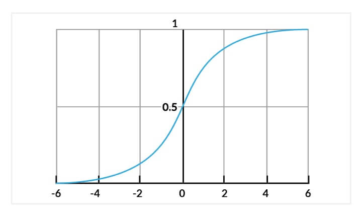
Logistic regression algorithms are the go-to for binary classification problems. There are two types of logistic regression: binary (eg: Does an input belong to the default class? Yes/No) and multilinear (Does the input image contain a dog? A cat? A sheep?). The algorithm maps predicted values to probabilities using the Sigmoid function, an S-shaped curve also known as the logistic function. The function maps any real value onto another value between 0 and 1, which expresses the probability that an input belongs to the default class. Inputs are combined linearly using weights or coefficient values to predict an output value (y). The best coefficients result in a model that predicts a value very close to one for the default class and very close to zero for the other class.
For example, if we are modeling people’s sex as male or female from their height, then the first class could be male and the logistic regression model could be written as the probability of male given a person’s height, or:
P(sex=male|height) or P(X)=P(Y=1|X)
The probability prediction must be transformed into a binary value (0 or 1) in order to make a probability prediction.
What is it used for?
Logistic regression models are used for spam detection, fraud detection, and tumor image classification
3. Decision Tree
Decision trees are a type of supervised machine learning algorithm used for classification and regression problems in machine learning. With a flowchart-like structure, decision trees represent a sequential list of questions or features contained within a node. Each node branches into a subsequent node, with a final leaf node representing a class label (a decision taken after computing all features). In a decision tree, different features have different importance (represented by weights or percentages), and the relationships between them can be viewed easily. The paths from root to leaf represent classification rules. Decision trees come in two types: classification trees (yes/no types) or regression trees (continuous data types, such as a numerical value).
In decision analysis, a decision tree can be used to visually represent decisions and decision-making. When it comes to structured or tabular data, decision trees are considered the best method for model fitting.
What is it used for?
Decision tree algorithms are used for evaluating loan applications, risk assessments, fraud detection, and medical diagnosis.
4. Support Vector Machine (SVM)
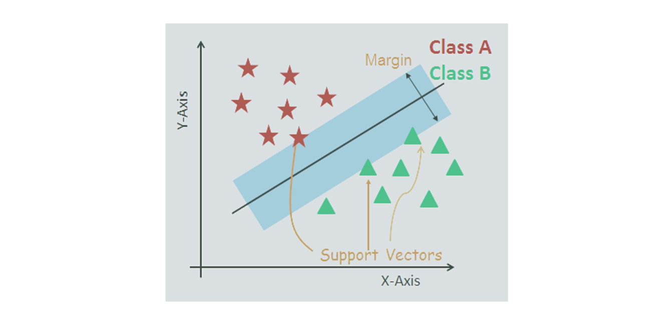
Support Vector Machine is a supervised machine learning algorithm used for classification and regression problems. The purpose of SVM is to find a hyperplane in an N-dimensional space (where N equals the number of features) that classifies the input data into distinct groups. The hyperplane represents a decision boundary, whereby the data points that fall on either side of it belong to a distinct class based on their shared similarities. Consequently, the objective of an SVM is to find a hyperplane that has the maximum margin (the maximum distance between data points of either class), in order to draw this distinction. SVM takes the data as an input, transforms it using a technique called the kernel tricks, and finds an optimal boundary (hyperplane) between the data points.
The dimension of the hyperplane depends on the number of features. If the number of input features is two, the hyperplane is just a line. However, if the number of features is three, the hyperplane becomes a two-dimensional plane. Support vectors are the data points closest to the hyperplane and influence the position and orientation of the hyperplane. We compute the distance (margin) between the hyperplane and the support vectors. Again, the goal is to maximize the margin. The hyperplane with the maximum margin between the data points of either class is the optimal hyperplane. SVM is considered a black box as the decisions and complex data transformations are very difficult to interpret.
What is it used for?
SVM is used for facial recognition, handwriting recognition, image classification, text categorization, and more.
5. Naive Bayes
Naive Bayes is a probabilistic classification algorithm based on the Bayes Theorem in statistics and probability theory. While this algorithm is used for a variety of classification tasks, it works especially well for natural language processing. The Bayes Theorem is a simple mathematical formula for calculating conditional probabilities. Conditional probability is the measure of the probability of an event given that another event has occurred. Essentially, the formula tells you how often A happens given B, expressed as P(A|B), or vice versa.
The fundamental Naive Bayes assumption is that each feature makes an independent and equal contribution to the outcome. For example, the condition of a fruit being red, round, and 2-4 inches in diameter are features that must all be present for it to be classified as an apple, but the algorithm perceives each feature as distinct. If given a sentence—for example, “the sky is blue”—the algorithm will interpret the individual words and not the entire sentence, even though words that stand next to each other in a sentence influence the meaning of the sentence. Hence why the algorithm is referred to as “naive.” Even though the independence assumption is generally incorrect in real-world situations, the Naive Bayes classifier is useful for large datasets because it works extremely fast relative to other classification algorithms, and has been known to outperform even highly sophisticated classification methods.
What is it used for?
Naive Bayes is used for image classification, document classification (eg: classifying texts into different languages, genres, or topics through the presence of keywords), and sentiment analysis (calculating the probability of a sentence or paragraph being positive or negative).
6. K-Nearest Neighbors (KNN)
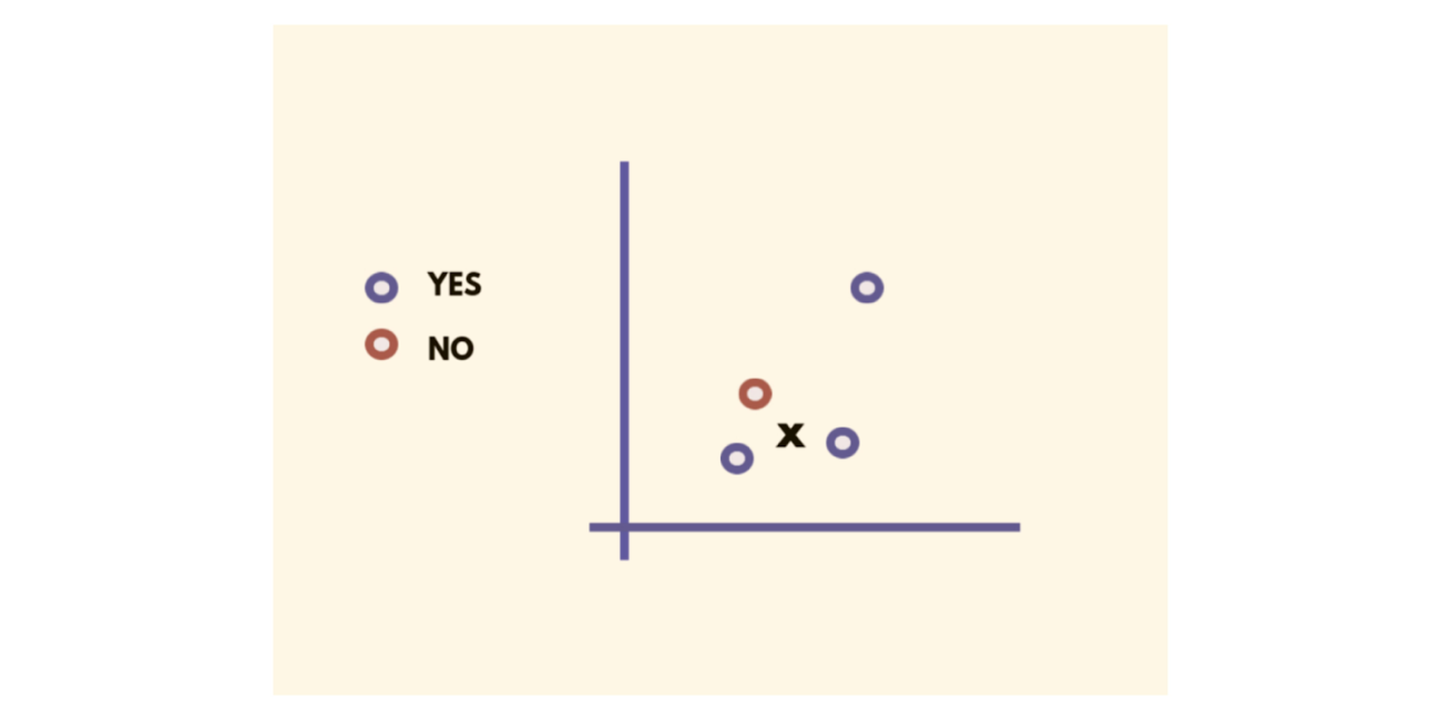
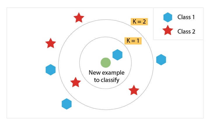
K-nearest neighbors is a supervised machine learning algorithm used to solve classification and regression problems. The algorithm assumes that similar data points exist in close proximity. KNN captures the idea of similarity by calculating the straight-line distance (AKA the Euclidean distance) between points on a graph. The algorithm then tries to establish nonlinear boundaries for each class, similar to an SVM. In KNN classification, an object is assigned to the class most common amongst its ‘k’ nearest neighbors, where k is a user-defined constant. Increasing k (up to a point) results in more stable predictions due to majority voting/averaging, and the algorithm is thus more likely to make accurate predictions. When k=1, the object is simply assigned to the class of its single nearest neighbor. Increasing k is akin to casting a wider fishing net, where the average is computed from a larger, more representative sample of “fish.” In KNN regression, the output is the property value for the object—meaning the value of all the average values of the K-nearest neighbors.
It is useful to assign weights to the contributions of the neighbors so that the nearest neighbors contribute more to the average than distant ones. This also prevents bias when the class distribution is skewed. Samples of a more prevalent class tend to dominate the prediction of a new example because they tend to be common among the k-nearest neighbors due to their large number.
KNN works by finding the distances between a query and all the examples in the data, selecting the specified number of examples (k) closest to the query, then voting for the most frequent label (in the case of classification) or averaging the labels (in the case of regression).
What is it used for?
KNN is used in recommender systems, such as products on Amazon, movies on Netflix, and videos on YouTube.
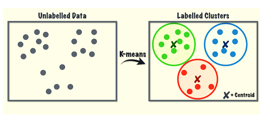
7. K-Means
K-means is a method of vector quantization that aims to separate n observations into k clusters. Unlike KNN, K-Means is used to find groups that have not been explicitly labeled in the data. Clustering is one of the most common exploratory data analysis techniques because it can be used to find out what groups exist or to identify unknown groups from complex datasets. Clustering is the process of identifying non-overlapping subgroups (clusters) within the data such that the data points in the same cluster are very similar, while the data points in other clusters are very different (i.e. far apart according to Euclidean distance or correlation-based distance). The objective of K-means is to group similar data points together and discover underlying patterns.
The target number, k, refers to the number of centroids you need in the dataset. A centroid represents the center of the cluster—the arithmetic mean of every data point that belongs to that cluster. The algorithm attempts to minimize the sum of the squared distance between data points and the centroid.
Clustering can be done based on subgroups or features. Since clustering algorithms use distance-based measurements to determine the similarity between data points, it’s best to standardize the data to have a mean of zero and a standard deviation of one. In most datasets, the features have different units of measurement (eg: height vs. weight), so these units must be standardized.
What is it used for?
K-means is used for market segmentation when we try to find customers that are similar to each in terms of behavior/attributes, image recognition, and document clustering.
8. Random Forest
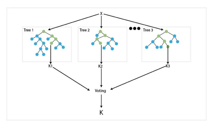
Random forest is a supervised learning algorithm used for classification, regression, and other tasks. The algorithm consists of a multitude of decision trees—known as a “forest”—which have been trained with the bagging method. The general idea of the bagging method is that a combination of learning models increases the accuracy of the overall result. This method is known as ensemble learning, a technique that combines many classifiers to provide solutions to complex problems. Random forest builds multiple decision trees and merges their outputs (predictions) by taking the mean or average of all the outputs to obtain a more stable and accurate prediction.
In every random forest, a subset of features is selected randomly at each node’s splitting point, where the randomized feature selection reduces bias. Consequently, random forest overcomes the limitations of the decision tree algorithm by reducing overfitting of datasets and increasing precision.
9. Dimensionality reduction
Dimensionality reduction algorithms are used for feature selection and feature extraction. In machine learning classification problems, there are often too many variables that form the basis of a classification. These variables are called features. The higher the number of features, the harder it is to make predictions from the training set. Oftentimes, most of these features are correlated, hence redundant. For example, if 95% of observations were for 35-year-old women, then age and gender variables can be eliminated without losing too much information. Some features have nothing to do with the target variable; others might be correlated to the target variable but have no causal relationship to it.
If redundancies aren’t eliminated, models will try to map any feature included in the dataset to the target variable even if there is no relationship between them, which leads to imprecision.
Dimensionality reduction is the process of reducing the number of random variables under consideration and instead of obtaining a set of principal variables. In machine learning, dimensionality refers to the number of features in your dataset. When there’s an insufficient number of observations for each feature, the algorithm may struggle to train models effectively because the model doesn’t have enough samples for each feature. This is known as the “curse of dimensionality” and is especially relevant for clustering algorithms that rely on distance calculations.
Feature selection refers to filtering irrelevant or redundant features from your dataset, while feature extraction involves compressing near-identical features into a lower-dimensional space.
What is it used for?
Dimensionality reduction is a necessary procedure when working with large datasets because it results in data compression, hence reduced storage space and computing power.
10. Gradient boosting algorithms
Gradient boosting algorithms are another example of ensemble learning, where weak prediction models are combined to create a more powerful new model. Boosting is a method for creating an ensemble. It starts by fitting an initial model, such as a tree or linear regression, to the data. Then a second model is created to predict the cases where the first model performs poorly. This process is repeated many times, where each subsequent model attempts to correct the shortcomings of the combined boosted ensemble of all previous models.
A weak model refers to one whose performance is slightly better than random chance. Gradient boosting is one of the most powerful algorithms in the field of machine learning. It refers to a family of machine learning algorithms that convert weak learners into stronger models in an iterative process.
The term ‘gradient boosting’ refers to the use of a gradient descent algorithm to minimize the loss when adding new models. Target outcomes for each case are set based on the gradient of the error with respect to the prediction. XGBoost
11. XGBoost
XGBoost is a decision tree algorithm that uses a gradient boosting framework. Developed as a research project at the University of Washington, XGBoost is the most popular gradient boosting R package and has been widely used in cutting-edge industry applications and Kaggle competitions. XGBoost, which stands for “Extreme Gradient Boosting,” is an optimized distributed gradient boosting library designed to be more efficient, flexible, and portable than gradient boosted decision trees. Features of XGBoost include regularized learning, which helps to smooth the final learned weights to avoid model overfitting. Also, the tree ensemble cannot be optimized using traditional optimization methods such as Euclidean space (the distance measure that determines accuracy in classification models), so the model is trained in an additive manner.
As an open-source implementation tool, XGBoost belongs to a broader collection of tools under the Distributed (Deep) Machine Learning Community on GitHub.
What is it used for?
According to the researchers who came up with it, the most important factor about the XGBoost is its scalability and speed, with a system that runs more than 10x faster than existing popular solutions on a single machine while enabling data scientists to process hundreds of millions of examples on a standard desktop computer.
12. GBM (Gradient Boosting Machine)
Gradient Boosting Machine is the original gradient boosting framework for decision trees introduced in 2001 by Jerome H. Friedman, a professor of statistics at Stanford University. Also known as MART (Multiple Additive Regression Trees) and GBRT (Gradient Boosted Regression Trees). GBM identifies weak learners by using gradients in the loss function (y=ax+b+e, where e is the error term). The loss function measures how good a model’s coefficients are at fitting the underlying data. Put more simply, the loss function indicates the difference between true values and predicted values.
13. LightGBM
Another free and open-source gradient boosting framework for decision tree algorithms, LightGBM was initially developed by Microsoft. LightGBM has many of the same advantages as XGBoost, including sparse organization, parallel training (training different layers of a model on different GPUs to reduce training time), multiple loss functions, regularization (a technique used for tuning the function) , and early stopping.
The main difference between XGBoost and LightGBM lies in the construction of the decision trees. LightGBM does not grow a tree row by row as most other implementations do. Instead, it chooses the leaf (terminal node) it believes will yield the largest decrease in loss (which is the main objective of gradient boosting). Comparison experiments on public datasets show that LightGBM can outperform existing boosting frameworks such as XGBoost on both efficiency and accuracy, with lower memory consumption.
14. CatBoost
Yet another open-source gradient boosting library for decision trees, CatBoost was developed by researchers and engineers at Yandex, a Russian-Dutch internet company. The library is used for search, recommendation systems, personal assistants, self-driving cars, weather prediction, and many other tasks at Yandex and other companies.
Cloudflare, a web security company, used the CatBoost algorithm to build a machine learning model that would counteract credential stuffing bots—cyberattacks that attempt to log into and take over a user’s account by assaulting password forms with previously stolen credentials. CatBoost provides great results with default parameters, so there is no need to spend too much time on parameter tuning. You can also use non-numeric factors instead of having to pre-process your data and turn it into numbers.
What Are the Best Machine Learning Algorithms?
Machine learning enables businesses to analyze massive datasets to gain insights about their customers, make forecasts about future events, and provide a personalized customer experience. Fundamentally, machine learning extracts meaningful insights from raw data to solve complex business problems. However, no one machine learning algorithm works best for every problem—hence the concept of the “no free lunch” theorem in supervised machine learning. Predictive analytics is the most common type of machine learning, which involves the mapping Y=f(x) to make predictions of Y for new X. Linear regression is widely used for predicting sales revenue, setting prices, and analyzing risk in the financial and insurance sectors.
The “best” algorithms to use varies widely by industry, depending on the nature of the business problem and the type of data available. For example, image recognition is becoming increasingly prevalent in healthcare for its usefulness in medical diagnostics, such as classifying an MRI of a brain tumor as benign or malignant—an example of a binary classification problem that can be solved using logistic regression. Meanwhile, retailers use a range of machine learning algorithms from simple linear regression to Naive Bayes to improve inventory control using predictive analytics, perform sentiment analysis to predict the likelihood of customer churn, and using K-means clustering for customer segmentation.
Meanwhile, the financial and insurance industries use decision trees and corresponding gradient boosting libraries such as XGBoost, CatBoost, and GBM to evaluate loan and mortgage applications, detect fraud, and perform risk assessments before entering new markets. While some algorithms are used more than others in certain industries, every type of algorithm has a significant role to play in developing machine learning models that are more accurate and less prone to bias.
Though we’re living through a time of extraordinary innovation in GPU-accelerated machine learning, the latest research papers frequently (and prominently) feature algorithms that are decades, in certain cases 70 years old.
Some might contend that many of these older methods fall into the camp of ‘statistical analysis’ rather than machine learning, and prefer to date the advent of the sector back only so far as 1957, with the invention of the Perceptron.
Given the extent to which these older algorithms support and are enmeshed in the latest trends and headline-grabbing developments in machine learning, it’s a contestable stance. So let’s take a look at some of the ‘classic’ building blocks underpinning the latest innovations, as well as some newer entries that are making an early bid for the AI hall of fame.
1: Transformers
In 2017 Google Research led a research collaboration culminating in the paper Attention Is All You Need. The work outlined a novel architecture that promoted attention mechanisms from ‘piping’ in encoder/decoder and recurrent network models to a central transformational technology in their own right.
The approach was dubbed Transformer, and has since become a revolutionary methodology in Natural Language Processing (NLP), powering, amongst many other examples, the autoregressive language model and AI poster-child GPT-3.
Transformers elegantly solved the problem of sequence transduction, also called ‘transformation’, which is occupied with the processing of input sequences into output sequences. A transformer also receives and manages data in a continuous manner, rather than in sequential batches, allowing a ‘persistence of memory’ which RNN architectures are not designed to obtain. For a more detailed overview of transformers, take a look at our reference article.
In contrast to the Recurrent Neural Networks (RNNs) that had begun to dominate ML research in the CUDA era, Transformer architecture could also be easily parallelized, opening the way to productively address a far larger corpus of data than RNNs.
Popular Usage
Transformers captured the public imagination in 2020 with the release of OpenAI’s GPT-3, which boasted a then record-breaking 175 billion parameters. This apparently staggering achievement was eventually overshadowed by later projects, such as the 2021 release of Microsoft’s Megatron-Turing NLG 530B, which (as the name suggests) features over 530 billion parameters.
A timeline of hyperscale Transformer NLP projects. Source: Microsoft
Transformer architecture has also crossed over from NLP to computer vision, powering a new generation of image synthesis frameworks such as OpenAI’s CLIP and DALL-E, which use text>image domain mapping to finish incomplete images and synthesize novel images from trained domains, among a growing number of related applications.
DALL-E attempts to complete a partial image of a bust of Plato. Source: https://openai.com/blog/dall-e/
2: Generative Adversarial Networks (GANs)
Though transformers have gained extraordinary media coverage through the release and adoption of GPT-3, the Generative Adversarial Network (GAN) has become a recognizable brand in its own right, and may eventually join deepfake as a verb.
First proposed in 2014 and primarily used for image synthesis, a Generative Adversarial Network architecture is composed of a Generator and a Discriminator. The Generator cycles through thousands of images in a dataset, iteratively attempting to reconstruct them. For each attempt, the Discriminator grades the Generator’s work, and sends the Generator back to do better, but without any insight into the way that the previous reconstruction erred.
This forces the Generator to explore a multiplicity of avenues, instead of following the potential blind alleys that would have resulted if the Discriminator had told it where it was going wrong (see #8 below). By the time the training is over, the Generator has a detailed and comprehensive map of relationships between points in the dataset.
From the paper Improving GAN Equilibrium by Raising Spatial Awareness: a novel framework cycles through the sometimes-mysterious latent space of a GAN, providing responsive instrumentality for an image synthesis architecture. Source: https://genforce.github.io/eqgan/
By analogy, this is the difference between learning a single humdrum commute to central London, or painstakingly acquiring The Knowledge.
The result is a high-level collection of features in the latent space of the trained model. The semantic indicator for a high level feature could be ‘person’, whilst a descent through specificity related to the feature may unearth other learned characteristics, such as ‘male’ and ‘female’. At lower levels the sub-features can break down to, ‘blonde’, ‘Caucasian’, et al.
Entanglement is a notable issue in the latent space of GANs and encoder/decoder frameworks: is the smile on a GAN-generated female face an entangled feature of her ‘identity’ in the latent space, or is it a parallel branch?
GAN-generated faces from thispersondoesnotexist. Source: https://this-person-does-not-exist.com/en
The past couple of years have brought forth a growing number of new research initiatives in this respect, perhaps paving the way for feature-level, Photoshop-style editing for the latent space of a GAN, but at the moment, many transformations are effectively ‘all or nothing’ packages. Notably, NVIDIA’s EditGAN release of late 2021 achieves a high level of interpretability in the latent space by using semantic segmentation masks.
Popular Usage
Beside their (actually fairly limited) involvement in popular deepfake videos, image/video-centric GANs have proliferated over the last four years, enthralling researchers and the public alike. Keeping up with the dizzying rate and frequency of new releases is a challenge, though the GitHub repository Awesome GAN Applications aims to provide a comprehensive list.
Generative Adversarial Networks can in theory derive features from any well-framed domain, including text.
3: SVM
Originated in 1963, Support Vector Machine (SVM) is a core algorithm that crops up frequently in new research. Under SVM, vectors map the relative disposition of data points in a dataset, while support vectors delineate the boundaries between different groups, features, or traits.
Support vectors define the boundaries between groups. Source: https://www.kdnuggets.com/2016/07/support-vector-machines-simple-explanation.html
The derived boundary is called a hyperplane.
At low feature levels, the SVM is two-dimensional (image above), but where there’s a higher recognized number of groups or types, it becomes three-dimensional.
A deeper array of points and groups necessitates a three-dimensional SVM. Source: https://cml.rhul.ac.uk/svm.html
Popular Usage
Since support Vector Machines can effectively and agnostically address high-dimensional data of many kinds, they crop up widely across a variety of machine learning sectors, including deepfake detection, image classification, hate speech classification, DNA analysis and population structure prediction, among many others.
4: K-Means Clustering
Clustering in general is an unsupervised learning approach that seeks to categorize data points through density estimation, creating a map of the distribution of the data being studied.
K-Means clustering divines segments, groups and communities in data. Source: https://aws.amazon.com/blogs/machine-learning/k-means-clustering-with-amazon-sagemaker/
K-Means Clustering has become the most popular implementation of this approach, shepherding data points into distinctive ‘K Groups’, which may indicate demographic sectors, online communities, or any other possible secret aggregation waiting to be discovered in raw statistical data.
The K value itself is the determinant factor in the utility of the process, and in establishing an optimal value for a cluster. Initially, the K value is randomly assigned, and its features and vector characteristics compared to its neighbors. Those neighbors that most closely resemble the data point with the randomly assigned value get assigned to its cluster iteratively until the data has yielded all the groupings that the process permits.
The plot for the squared error, or ‘cost’ of differing values among the clusters will reveal an elbow point for the data:
The elbow point is similar in concept to the way that loss flattens out to diminishing returns at the end of a training session for a dataset. It represents the point at which no further distinctions between groups is going to become apparent, indicating the moment to move on to subsequent phases in the data pipeline, or else to report findings.
Popular Usage
K-Means Clustering, for obvious reasons, is a primary technology in customer analysis, since it offers a clear and explainable methodology to translate large quantities of commercial records into demographic insights and ‘leads’.
Outside of this application, K-Means Clustering is also employed for landslide prediction, medical image segmentation, image synthesis with GANs, document classification, and city planning, among many other potential and actual uses.
5: Random Forest
Random Forest is an ensemble learning method that averages the result from an array of decision trees to establish an overall prediction for the outcome.
If you’ve researched it even as little as watching the Back to the Future trilogy, a decision tree itself is fairly easy to conceptualize: a number of paths lie before you, and each path branches out to a new outcome which in turn contains further possible paths.
In reinforcement learning, you might retreat from a path and start again from an earlier stance, whereas decision trees commit to their journeys.
Thus the Random Forest algorithm is essentially spread-betting for decisions. The algorithm is called ‘random’ because it makes ad hoc selections and observations in order to understand the median sum of the results from the decision tree array.
Since it takes into account a multiplicity of factors, a Random Forest approach can be more difficult to convert into meaningful graphs than a decision tree, but is likely to be notably more productive.
Decision trees are subject to overfitting, where the results obtained are data-specific and not likely to generalize. Random Forest’s arbitrary selection of data points combats this tendency, drilling through to meaningful and useful representative trends in the data.
Popular Usage
As with many of the algorithms in this list, Random Forest typically operates as an ‘early’ sorter and filter of data, and as such consistently crops up in new research papers. Some examples of Random Forest usage include Magnetic Resonance Image Synthesis, Bitcoin price prediction, census segmentation, text classification and credit card fraud detection.
Since Random Forest is a low-level algorithm in machine learning architectures, it can also contribute to the performance of other low-level methods, as well as visualization algorithms, including Inductive Clustering, Feature Transformations, classification of text documents using sparse features, and displaying Pipelines.
6: Naive Bayes
Coupled with density estimation (see 4, above), a naive Bayes classifier is a powerful but relatively lightweight algorithm capable of estimating probabilities based on the calculated features of data.
The term ‘naïve’ refers to the assumption in Bayes’ theorem that features are unrelated, known as conditional independence. If you adopt this standpoint, walking and talking like a duck aren’t enough to establish that we’re dealing with a duck, and no ‘obvious’ assumptions are prematurely adopted.
This level of academic and investigative rigor would be overkill where ‘common sense’ is available, but is a valuable standard when traversing the many ambiguities and potentially unrelated correlations that may exist in a machine learning dataset.
In an original Bayesian network, features are subject to scoring functions, including minimal description length and Bayesian scoring, which can impose restrictions on the data in terms of the estimated connections found between the data points, and the direction in which these connections flow.
A naive Bayes classifier, conversely, operates by assuming that the features of a given object are independent, subsequently using Bayes’ theorem to calculate the probability of a given object, based on its features.
Popular Usage
Naive Bayes filters are well-represented in disease prediction and document categorization, spam filtering, sentiment classification, recommender systems, and fraud detection, among other applications.
7: K- Nearest Neighbors (KNN)
First proposed by the US Air Force School of Aviation Medicine in 1951, and having to accommodate itself to the state-of-the-art of mid-20th century computing hardware, K-Nearest Neighbors (KNN) is a lean algorithm that still features prominently across academic papers and private sector machine learning research initiatives.
KNN has been called ‘the lazy learner’, since it exhaustively scans a dataset in order to evaluate the relationships between data points, rather than requiring the training of a full-fledged machine learning model.
Though KNN is architecturally slender, its systematic approach does place a notable demand on read/write operations, and its use in very large datasets can be problematic without adjunct technologies such as Principal Component Analysis (PCA), which can transform complex and high volume datasets into representative groupings that KNN can traverse with less effort.
A recent study evaluated the effectiveness and economy of a number of algorithms tasked to predict whether an employee will leave a company, finding that the septuagenarian KNN remained superior to more modern contenders in terms of accuracy and predictive effectiveness.
Popular Usage
For all its popular simplicity of concept and execution, KNN is not stuck in the 1950s – it’s been adapted into a more DNN-focused approach in a 2018 proposal by Pennsylvania State University, and remains a central early-stage process (or post-processing analytical tool) in many far more complex machine learning frameworks.
In various configurations, KNN has been used or for online signature verification, image classification, text mining, crop prediction, and facial recognition, besides other applications and incorporations.
8: Markov Decision Process (MDP)
A mathematical framework introduced by American mathematician Richard Bellman in 1957, The Markov Decision Process (MDP) is one of the most basic blocks of reinforcement learning architectures. A conceptual algorithm in its own right, it has been adapted into a great number of other algorithms, and recurs frequently in the current crop of AI/ML research.
MDP explores a data environment by using its evaluation of its current state (i.e. ‘where’ it is in the data) to decide which node of the data to explore next.
A basic Markov Decision Process will prioritize near-term advantage over more desirable long-term objectives. For this reason, it is usually embedded into the context of a more comprehensive policy architecture in reinforcement learning, and is often subject to limiting factors such as discounted reward, and other modifying environmental variables that will prevent it from rushing to an immediate goal without consideration of the broader desired outcome.
Popular Usage
MDP’s low-level concept is widespread in both research and active deployments of machine learning. It’s been proposed for IoT security defense systems, fish harvesting, and market forecasting.
Besides its obvious applicability to chess and other strictly sequential games, MDP is also a natural contender for the procedural training of robotics systems, as we can see in the video below.
Global Planner using a Markov Decision Process – Mobile Industrial Robotics
9: Term Frequency-Inverse Document Frequency
Term Frequency (TF) divides the number of times a word appears in a document by the total number of words in that document. Thus the word seal appearing once in a thousand-word article has a term frequency of 0.001. By itself, TF is largely useless as an indicator of term importance, due to the fact that meaningless articles (such as a, and, the, and it) predominate.
To obtain a meaningful value for a term, Inverse Document Frequency (IDF) calculates the TF of a word across multiple documents in a dataset, assigning low rating to very high-frequency stopwords, such as articles. The resulting feature vectors are normalized to whole values, with each word assigned an appropriate weight.
TF-IDF weights the relevance of terms based on frequency across a number of documents, with rarer occurrence an indicator of salience. Source: https://moz.com/blog/inverse-document-frequency-and-the-importance-of-uniqueness
Though this approach prevents semantically important words from being lost as outliers, inverting the frequency weight does not automatically mean that a low-frequency term is not an outlier, because some things are rare and worthless. Therefore a low-frequency term will need to prove its value in the wider architectural context by featuring (even at a low frequency per document) in a number of documents in the dataset.
Despite its age, TF-IDF is a powerful and popular method for initial filtering passes in Natural Language Processing frameworks.
Popular Usage
Because TF-IDF has played at least some part in the development of Google’s largely occult PageRank algorithm over the last twenty years, it has become very widely adopted as a manipulative SEO tactic, in spite of John Mueller’s 2019 disavowal of its importance to search results.
Due to the secrecy around PageRank, there is no clear evidence that TF-IDF is not currently an effective tactic for rising in Google’s rankings. Incendiary discussion among IT professionals lately indicates a popular understanding, correct or not, that term abuse may still result in improved SEO placement (though additional accusations of monopoly abuse and excessive advertising blur the confines of this theory).
10: Stochastic Gradient Descent
Stochastic Gradient Descent (SGD) is an increasingly popular method for optimizing the training of machine learning models.
Gradient Descent itself is a method of optimizing and subsequently quantifying the improvement that a model is making during training.
In this sense, ‘gradient’ indicates a slope downwards (rather than a color-based gradation, see image below), where the highest point of the ‘hill’, on the left, represents the beginning of the training process. At this stage the model has not yet seen the entirety of the data even once, and has not learned enough about relationships between the data to produce effective transformations.
A gradient descent on a FaceSwap training session. We can see that the training has plateaued for some time in the second half, but has eventually recovered its way down the gradient towards an acceptable convergence.
The lowest point, on the right, represents convergence (the point at which the model is as effective as it is ever going to get under the imposed constraints and settings).
The gradient acts as a record and predictor for the disparity between the error rate (how accurately the model has currently mapped the data relationships) and the weights (the settings that influence the way in which the model will learn).
This record of progress can be used to inform a learning rate schedule, an automatic process that tells the architecture to become more granular and precise as the early vague details transform into clear relationships and mappings. In effect, gradient loss provides a just-in-time map of where the training should go next, and how it should proceed.
The innovation of Stochastic Gradient Descent is that it updates the model’s parameters on each training example per iteration, which generally speeds up the journey to convergence. Due to the advent of hyperscale datasets in recent years, SGD has grown in popularity lately as one possible method to address the ensuing logistic issues.
On the other hand, SGD has negative implications for feature scaling, and may require more iterations to achieve the same result, requiring additional planning and additional parameters, compared to regular Gradient Descent.
Popular Usage
Due to its configurability, and in spite of its shortcomings, SGD has become the most popular optimization algorithm for fitting neural networks. One configuration of SGD that is becoming dominant in new AI/ML research papers is the choice of the Adaptive Moment Estimation (ADAM, introduced in 2015) optimizer.
ADAM adapts the learning rate for each parameter dynamically (‘adaptive learning rate’), as well as incorporating results from previous updates into the subsequent configuration (‘momentum’). Additionally, it can be configured to use later innovations, such as Nesterov Momentum.
However, some maintain that the use of momentum can also speed ADAM (and similar algorithms) to a sub-optimal conclusion. As with most of the bleeding edge of the machine learning research sector, SGD is a work in progress.
Machine learning is the most ideal choice for not only the financial technology domain, which algorithmic trading is a part of, but also for other industries such as healthcare, retail, education, etc.
Alan Turing, an English mathematician, computer scientist, logician, and cryptanalyst, surmised about machines that, “It would be like a pupil who had learnt much from his master but had added much more by his own work. When this happens I feel that one is obliged to regard the machine as showing intelligence.”
This blog is a comprehensive guide to help you understand the basic logic behind some popular and incredibly resourceful machine learning algorithms for beginners used by the trading community, this blog is your one stop shop.
These machine learning algorithms for beginners also serve as the foundation stone for creating some of the best algorithms.
This blog covers the following:
Machine learning in brief
Types of machine learning algorithms
Top 10 machine learning algorithms for beginners
Honourable mentions
How to choose the machine learning algorithm?
Machine learning in brief
Machine learning, as the name suggests, is the ability of a machine to learn, even without programming it explicitly. It is a type of Artificial Intelligence which is based on algorithms to detect patterns in data and adjust the program actions accordingly.
Let us understand the machine learning concept with an example.
It is well known that Facebook’s News feed personalised each of its members’ feed using artificial intelligence or let us say machine learning. The software uses statistical and predictive analytics to identify patterns in the user’s data and uses it to populate the user’s Newsfeed.
If a user reads and comments on a particular friend’s posts then the news feed will be designed in a way that more activities of that particular friend will be visible to the user in his feed. The advertisements are also shown in the feed according to the data based on the user’s interests, likes, and comments on Facebook pages.
Components of machine learning algorithms
1. Representation: It includes the representation of data. It is done through decision trees, neural networks, support vector machines, regressions and others.
2. Evaluation: It is the way to evaluate programs. It involves accuracy, probability, squared error, margin, and others.
3. Optimization: It is the way programs are generated and it uses combinatorial optimization, convex optimization, and constrained optimization.
Types of machine learning algorithms
The types of machine learning algorithms are divided into 4 main categories, which are:
Supervised
Semi-supervised
Unsupervised
Reinforcement learning
Supervised
In supervised learning, the machine learns with the help of information provided manually. This information is imparted to the machine with the help of examples. The machine is fed the desired inputs and outputs manually. After learning from the fed information, the machine must find a method to determine how to arrive at those inputs and outputs.
The machine is fed the information via algorithms and with this information, the machine identifies patterns in data, learns from the observations and makes predictions. The machine makes predictions and is corrected manually in case of any mistakes. This process of trial and error continues until the machine achieves a high level of accuracy/performance.
In the case of supervised machine learning, there are these two types:
Classification – The machine is fed the data with different categories. In the case of classification, the machine learns which category the new data go to.
For instance, the categories in the data fed to the machine can be stock prices and returns. The machine learns to filter the data into the stock price and returns by looking at the existing observational data.
Regression – A regression implies the statistical relation of the dependent variable to one or more independent variables. The regression model shows whether the changes in the dependent variable are associated with the changes in one or more independent variables. Independent variables are also known as ‘predictors’, ‘covariates’, ‘explanatory variables’ or ‘features’.
For instance, the stock price is the dependent variable whereas the returns is the independent variable. Any changes in the dependent variable, that is, the stock price will lead to a change in the independent variable, that is, the returns.
Semi-supervised
Semi-supervised learning is similar to supervised learning. In the case of semi-supervised learning, the machine learns with the help of both labelled and unlabelled data. Labelled data holds the critical information so that the algorithm can understand the data, whilst unlabelled data lacks that information. By using the permutations and combinations of the labelled data, machine learning algorithms can learn to label the unlabelled data independently.
Unsupervised
Unsupervised learning is a type of machine learning in which only the input data is provided and the output data (labelling) is absent. Algorithms in unsupervised learning are left on their own without any assistance, to find results on their own and in this method of learning there are no correct or wrong answers.
Some of the popular unsupervised learning algorithms are:
Hierarchical clustering: builds a multilevel hierarchy of clusters by creating a cluster tree
k-Means clustering: partitions data into k distinct clusters based on the distance to the centroid of a cluster
Apriori algorithm: for association rule, learning problems
Reinforcement learning
The concept of reinforcement learning is as simple as being rewarded for the right choice while being punished for the wrong.
This concept is quite straightforward as the machine learns the permutations and combinations or the patterns for which it is rewarded (positive reinforcement) and discards the ones for which it is punished (negative reinforcement).
In the case of reinforcement learning, you don’t have to provide labels at each time step to the machine. The machine initially learns to trade through trial and error and receives a reward when the trade is closed. Later, the machine optimises the strategy to maximise the rewards.
Top 10 machine learning algorithms for beginners
We will now discuss the top 10 machine learning algorithms for beginners, which are:
Linear Regression
Logistic regression
KNN Classification
Support Vector Machine (SVM)
Decision Trees
Random Forest
Artificial Neural Network
K-means Clustering
Naive Bayes theorem
Recurrent Neural Networks (RNN)
Linear Regression
Initially developed in statistics to study the relationship between input and output numerical variables, it was adopted by the machine learning community to make predictions based on the linear regression equation.
The mathematical representation of linear regression is a linear equation that combines a specific set of input data (x) to predict the output value (y) for that set of input values. The linear equation assigns a factor to each set of input values, which are called the coefficients represented by the Greek letter Beta (β).
The equation mentioned below represents a linear regression model with two sets of input values, x1 and x2. y represents the output of the model, β0, β1 and β2 are the coefficients of the linear equation.
y = β0 + β1×1 + β2×2
When there is only one input variable, the linear equation represents a straight line. For simplicity, consider β2 to be equal to zero, which would imply that the variable x2 will not influence the output of the linear regression model. In this case, the linear regression will represent a straight line and its equation is shown below.
y = β0 + β1×1
A graph of the linear regression equation model is shown below.
Linear regression
Linear regression can be used to find the general price trend of a stock over a period of time. This helps us understand if the price movement is positive or negative.
Logistic regression
In logistic regression, our aim is to produce a discrete value, either 1 or 0. This helps us in finding a definite answer to our scenario.
Logistic regression can be mathematically represented as,
The logistic regression model computes a weighted sum of the input variables similar to the linear regression, but it runs the result through a special non-linear function, the logistic function or sigmoid function to produce the output y.
The sigmoid/logistic function is given by the following equation:
y = 1 / (1+ e-x)
Sigmoid function
In simple terms, logistic regression can be used to predict the direction of the market.
KNN Classification
The purpose of the K nearest neighbours (KNN) classification is to separate the data points into different classes so that we can classify them based on similarity measures (e.g. distance function).
KNN learns as it goes, in the sense, it does not need an explicit training phase and starts classifying the data points decided by a majority vote of its neighbours.
The object is assigned to the class which is most common among its k nearest neighbours.
Let’s consider the task of classifying a green circle into class 1 and class 2. Consider the case of KNN based on the 1-nearest neighbour. In this case, KNN will classify the green circle into class 1.
Now let’s increase the number of nearest neighbours to 3 i.e., 3-nearest neighbours. As you can see in the figure there are ‘two’ class 2 objects and ‘one’ class 1 object inside the circle. KNN will classify a green circle into a class 2 object as it forms the majority.
KNN Classification
Support Vector Machine (SVM)
Support Vector Machine was initially used for data analysis. Initially, a set of training examples is fed into the SVM algorithm, belonging to one or the other category. The algorithm then builds a model that starts assigning new data to one of the categories that it has learned in the training phase.
In the SVM algorithm, a hyperplane is created which serves as a demarcation between the categories. When the SVM algorithm processes a new data point and depending on the side on which it appears it will be classified into one of the classes.
SVM
When related to trading, an SVM algorithm can be built which categorises the equity data as favourable buy, sell or neutral classes and then classifies the test data according to the rules.
Decision Trees
Decision trees are basically tree-like support tools which can be used to represent a cause and its effect. Since one cause can have multiple effects, we list them down (quite like a tree with its branches).
Decision trees
We can build the decision tree by organising the input data and predictor variables, and according to some criteria that we will specify.
The disadvantage of decision trees is that they are prone to overfitting due to their inherent design structure.
Random Forest
A random forest algorithm was designed to address some of the limitations of decision trees.
Random Forest comprises decision trees which are graphs of decisions representing their course of action or statistical probability. These multiple trees are mapped to a single tree which is called Classification and Regression (CART) Model.
To classify an object based on its attributes, each tree gives a classification which is said to “vote” for that class. The forest then chooses the classification with the greatest number of votes. For regression, it considers the average of the outputs of different trees.
Random forest
Random Forest works in the following way:
Assume the number of cases as N. A sample of these N cases is taken as the training set.
Consider M to be the number of input variables, a number m is selected such that m < M. The best split between m and M is used to split the node. The value of m is held constant as the trees are grown.
Each tree is grown as large as possible.
By aggregating the predictions of n trees (i.e., majority votes for classification, the average for regression), predict the new data.
Artificial Neural Network
In our quest to play God, an artificial neural network is one of our crowning achievements. We have created multiple nodes which are interconnected to each other, as shown in the image, which mimics the nerons in our brain. In simple terms, each neuron takes in information through another neuron, performs work on it, and transfers it to another neuron as output.
Artificial neural network
Each circular node represents an artificial neuron and an arrow represents a connection from the output of one neuron to the input of another.
Neural networks can be more useful if we use it to find interdependencies between various asset classes, rather than trying to predict a buy or sell choice.
K-means Clustering
In this machine learning algorithm, the goal is to label the data points according to their similarity. Thus, we do not define the clusters prior to the algorithm but instead, the algorithm finds these clusters as it goes forward.
A simple example would be that given the data of football players, we will use K-means clustering and label them according to their similarity. Thus, these clusters could be based on the striker’s preference to score on free kicks or successful tackles, even when the algorithm is not given pre-defined labels to start with.
K-means clustering would be beneficial to traders who feel that there might be similarities between different assets which cannot be seen on the surface.
Naive Bayes theorem
Now, if you remember basic probability, you would know that Bayes theorem was formulated in a way where we assume we have prior knowledge of any event that is related to the former event.
For example, to check the probability that you will be late to the office, one would like to know if you face any traffic on the way.
However, the Naive Bayes classifier algorithm assumes that two events are independent of each other and thus, this simplifies the calculations to a large extent. Initially thought of as nothing more than an academic exercise, Naive Bayes has shown that it works remarkably well in the real world as well.
The Naive Bayes algorithm can be used to find simple relationships between different parameters without having complete data.
Recurrent Neural Networks (RNN)
Did you know Siri and Google Assistant use RNN in their programming? RNNs are essentially a type of neural network which have a memory attached to each node which makes it easy to process sequential data i.e. one data unit is dependent on the previous one.
A way to explain the advantage of RNN over a normal neural network is that we are supposed to process word character by character. If the word is “trading”, a normal neural network node would forget the character “t” by the time it moves to “d” whereas a recurrent neural network will remember the character as it has its own memory.
Honourable mentions
Apart from the top 10 machine learning algorithms that we discussed above, there are some others that we will discuss here
AdaBoost or Adaptive Boost
Gradient Boost
XGBoost
LightGBM
AdaBoost or Adaptive Boost
AdaBoost, or Adaptive Boost, is similar to Random Forests because several decision trees help with predictions in this type of machine learning algorithm. However, there are three unique featuresof AdaBoost, which are:
Stump
AdaBoost creates a forest of stumps rather than trees. A stump is a tree that is made of only one node and two leaves (as shown in the image above).
The stumps that are created are not equally weighed in the final decision (final prediction). Stumps that create more error will have less say in the final decision.
Lastly, the order in which the stumps are constructed is important, because each stump aims to reduce the errors that the previous stump(s) made.
Gradient Boost
Gradient Boost is also an ensemble algorithm that uses boosting methods to develop an enhanced predictor. In many ways, Gradient Boost is similar to AdaBoost, but there are some key differences:
Gradient Boost builds trees and not stumps. The tress usually have 8–32 leaves.
Gradient Boost views the boosting problem as an optimization problem, where it uses a loss function and tries to minimize the error. This is why it’s called Gradient boost, as it’s inspired by gradient descent.
Lastly, the trees are used to predict the residuals of the samples (predicted minus actual).
While the last point may have been confusing, all that you need to know is that Gradient Boost starts by building one tree to try to fit the data, and the subsequent trees built after with an aim to reduce the residuals (error).
It does this by concentrating on the areas where the existing learners performed poorly, similar to AdaBoost.
XGBoost
XGBoost is one of the most popular and widely used algorithms today because of its useful features. It is similar to Gradient Boost but has a few extra features to supplement the usefulness. These features are:
A proportional shrinking of leaf nodes (pruning) — used to improve the generalization of the model
Newton Boosting — provides a direct route to the minima than gradient descent, making it much faster
An extra randomization parameter — reduces the correlation between trees, ultimately improving the strength of the ensemble
Unique penalization of trees
LightGBM
If you thought XGBoost was the best algorithm out there, think again. LightGBM is another type of boosting algorithm that has been shown to be faster and sometimes more accurate than XGBoost.
What makes LightGBM different is that it uses a unique technique called Gradient-based One-Side Sampling (GOSS) to filter out the data instances to find a split value.
This is different from XGBoost which uses pre-sorted and histogram-based algorithms to find the best split.
Now that you have learnt about some popular machine learning algorithms for beginners, let us also find out how to choose the one that fits your requirements.
How to choose the machine learning algorithm?
These steps help you find out the relevant steps for choosing the machine learning algorithm fit for you:
Step 1 – Selecting the algorithm as per the goal
It is well understood now that machine learning solves the problem of reaching your goal. So, first of all, let us see what is your goal for which we are selecting the algorithm.
In case your goal is to find out which two stocks are co-integrated for a pairs trading strategy, you will feed the cointegration formula to the reinforcement algorithm. The reinforcement algorithm will select the co-integrated stocks as the reward will get triggered and discard others.
Similarly, if you want your machine learning algorithm to learn to pull the data for the mentioned stocks, you can simply feed the supervised algorithm with the data consisting of OHLCV values.
Step 2 – Find out the speed and training time
Well, this is an important step since it will define the speed of your algorithm and the time it takes to be trained.
But, would you even need an extremely fast processing algorithm even if it means lower quality of training and eventually, the predictions?
Hence, you must go for a proper time allocation and such an algorithm which takes optimal training time and also has an optimal speed.
Step 3 – The number of features and parameters should be set
In case you want the machine learning algorithm to be fed a lot of features and parameters, then you must give it as much time as well. The number of features and parameters will decide the complexity of your machine learning algorithm.
Also, the more features, the more time it will take to train. Hence, you must choose the algorithm with the capacity to train for a longer time with accurate data.
Conclusion
According to a study by Preqin, 1,360 quantitative funds are known to use computer models in their trading process, representing 9% of all funds. Firms organise cash prizes for an individual’s machine learning strategy if it makes money in the test phase and in fact, invests its own money and takes it in the live trading phase. Thus, in the race to be one step ahead of the competition, everyone, be it billion-dollar hedge funds or individual trade, all are trying to understand and implement machine learning in their trading strategies.
You can go through the AI in Trading course on Quantra to learn these algorithms in detail as well as apply them in live markets successfully and efficiently.
You can enrol in the learning track on Machine learning & Deep learning on Quantra which covers classification algorithms, performance measures in machine learning, hyper-parameters, and the building of supervised classifiers.