Types of Learning Styles for Machine Learning Algorithms
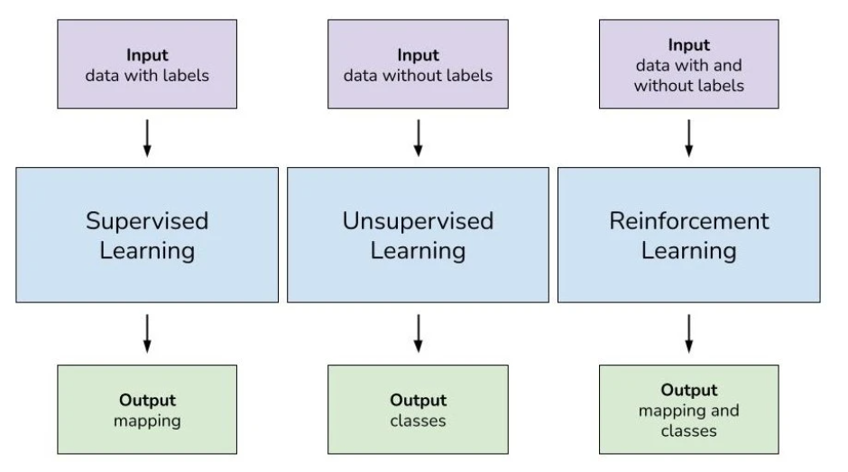
Before we begin discussing specific algorithms, however, we need a basic understanding of the different learning styles often seen in machine learning algorithms. These learning styles are supervised, unsupervised, and semi-supervised learning.
Types of Machine Learning and Differences Between Learning Styles
Supervised Learning
Supervised learning is a technique where a task is accomplished by providing training (input and output) patterns to the systems. Supervised learning in machine learning maps an input to its outputs based on sample input-output pairs. This type of learning infers a function from labeled and organized training data that consists of sets of training examples.
Datasets used for training with supervised learning are labeled with X and Y-axis variables and usually consist of metadata rather than image inputs. A popular example of a supervised learning dataset is the University of California Irvine Iris Dataset where the predicted attribute is the class of Iris (a type of flower) and the inputs are different variables depicting Iris classes (petal width and length, sepal width and length).
Supervised learning models are prepared through a training process where the model is required to make predictions and corrects itself when those predictions are incorrect. This guess-and-check type process continues until the model achieves a predetermined level of accuracy using the given training data.
Algorithms used for supervised learning are logistic regression and back propagation neural networks. Machine learning problems regarding supervised learning often involve classification and regression.
Unsupervised Learning
Unsupervised learning for machine learning does not require the creator to “supervise” the model during training. Unsupervised learning allows the model to discover patterns independently of a well-organized and labeled dataset. This is why unlabeled datasets are used often for unsupervised learning to generate machine learning models.
Unsupervised learning leaves algorithms to find structure in the inputs without the use of predefined variable names or labels.
While supervised learning models are given the inputs and left to predict the outputs, unsupervised learning models predict both the inputs and the outputs. This is done by detecting prominent patterns between inputs and associating those with potential outputs.
Algorithms specific to unsupervised machine learning models include K-means and the Apriori algorithm. Popular machine learning problems that can be solved using unsupervised learning involve clustering, dimensionality reduction, and association rule learning.
Semi-supervised Learning
Semi-supervised learning is the middle ground between unsupervised and supervised learning. Semi-supervised learning usually requires a combination of a small amount of labeled data and a comparatively large amount of unlabeled data for training its machine learning models.
As with supervised learning, example machine learning problems that can be solved with semi-supervised learning include classification and regressions. Semi-supervised learning is useful for image classification purposes but is still debated on whether it is the most efficient for that purpose.
Regression Algorithms for Machine Learning
Algorithms allow for sectors of machine learning like unsupervised, supervised, and semi-supervised learning to be productive.
Regression algorithms can be used for supervised and semi-supervised learning, and specifically deal with modeling the relationship between variables. It is refined iteratively using a measure of error in the predictions made by the model at hand. Regression is both a type of machine learning problem and algorithm.
For our intents and purposes, we are discussing regression as it relates to being a type of error-based machine learning algorithm. Popular regression algorithms include a handful, but the most relevant to us in this article are linear, logistic, and ordinary least squares regression.
Simple Linear Regression for Machine Learning
Regression is a method of modeling a target value based on independent predictors. This makes regression a good method for modeling a target value based on independent predictor variables.
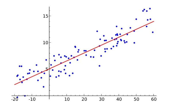
Linear regression for machine learning algorithms Simple linear regression is a relatively easy concept for a machine learning model algorithm in part due to its simplicity. The number of independent variables is 1, and there is a linear relationship between the independent and dependent X and Y variables. The line of best fit models given points in a dataset with the most accuracy. The line is then modeled with a linear equation where y = A0 + A1(x) → or y = mx + b.
Error Function
The error function (also known as “cost function”) is used to provide the “best” line of best fit for our respective data points. The search problem is converted into a minimization problem where the error between the predicted value and actual value is the least. In other words, the error function captures the error between the predictions made by a model versus the actual values in a training dataset.
Linear regression as an algorithm aims to find the best fitting values for A0 and A1 which is a two-part process that can be better understood by learning about cost function and gradient descent.
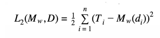
Sum of Squared Errors Error Function
The above mathematical representation is the formal definition of the sum of squared errors error function. Keep in mind that M is the complete machine learning model at hand, instead of a variable that represents a single value.
The training set given is composed of n training instances, each of which have d descriptive features and T single-target feature. Mw (d) is the prediction made by the candidate model at hand for any given training instance containing di descriptive features. The machine learning aspect of this function can be seen where the candidate model Mw is defined by the weight vector w.
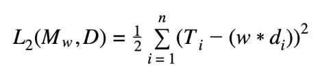
If we take, for example, a scenario where each instance is described with a single descriptive feature (meaning each independent data point maps to a singular dependent data point as the descriptive feature), the equation can expand to something like the following:
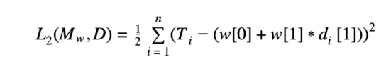
Expanded Error Function
The weights can change, there is a corresponding sum of squared errors value for every possible combination of weights (weights are also known as model parameters). The key to using simple linear regression models is determining the optimal values for the weights using the equation.
Error Surfaces to Find Optimal Values
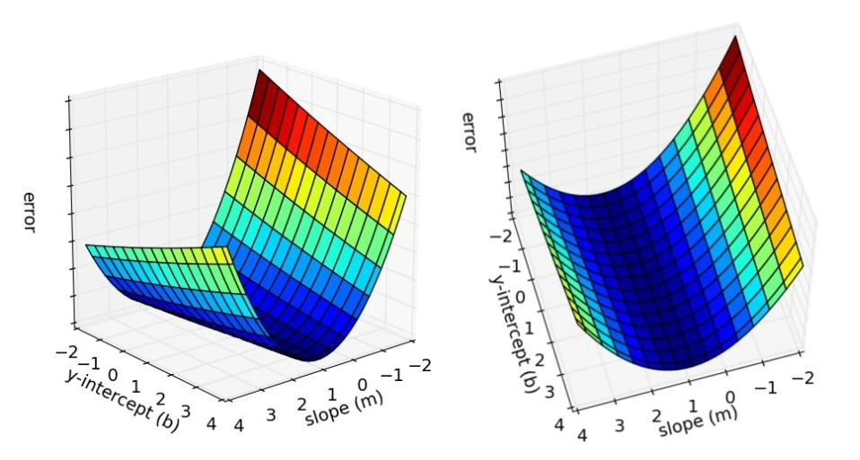
Error Surfaces to Determine Optimal Values The sum of squared errors function can be used to measure how well any combination of weights fits the respective instances in a dataset. Instead of using a brute-force search to find the best combination, we can use associated error surfaces to calculate the optimal combination of weights.
The error surfaces for any machine learning simple regression problem are convex (shaped like a bowl). We want to use the error surfaces to find a unique set of optimal weights with the lowest sum of squared errors (finding the global minimum). Finding the global minimum uses a process known as least squares optimization.
Least Squares Optimization
As mentioned earlier, we can predict that the error surface of our algorithm will produce a convex shape, thus possessing a global minimum. The distinctive shape of the error surfaces can be attributed to it being defined mostly by the linearity of the model, rather than the properties of the data. This means the partial derivatives of the error surface with respect to weights (w[0] and w[1]) are equal to 0 because they measure the slope of the error surface at the points w[0] and w[1].
The bottom of the error surface is not curved and does not have any slope, due to the convex shape, which is why the partial derivatives of the error surface are 0 at that point. We can infer that because of the aforementioned properties, that point is the global minimum of the error surface and are exactly the points we would need to calculate the most efficient weights to use for machine learning.
So how do we calculate the global minimum? By combining the equation discussed earlier for simple linear regression with partial derivatives, we can define the global minimum on the error surface as:
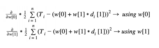
Global Minimum on the Error Surface
Multivariable Linear Regression with Gradient Descent
Multivariable linear regression with gradient descent can be used to train a best-fit model for a given training set and is one of the most common approaches to doing so within error-based machine learning.
It is still used only for supervised and semi-supervised learning because a dataset is required. While the simple linear regression section above dealt with a single descriptive feature, multivariable linear regression models can handle more than one descriptive features (and are thus, multivariable).
A random example of a machine learning model where this type of algorithm would be useful is for predicting the price of a house in a neighborhood where variables like land size, crime rate, and miles from schooling are integral to the fluctuating price of the house.
Multivariable Linear Regression Mathematical Representation
We can actually take our simple linear regression representation from earlier in the article and extend it to include an array of variables rather than just one.
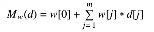
variables extended simple linear regression representation
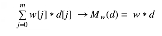
In this instance, d is the array of m descriptive features. Thus, d[1]…d[m] represents all descriptive features, while w[1]…w[m] are m+1 weights. We can then simplify the above expansion by using a nonexistent descriptive feature, d[0], which is equal to 1. This then produces:
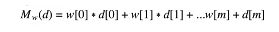
expanded simple linear regression representation
We can easily spot the summation process in this equation, so we can replace it with sigma, and reduce the sum of all descriptive features to just Mw(d) =w*d.
What this means, in essence, is that w*d is the sum of the products of the arrays’ w and d corresponding elements. The loss function calculated earlier (L2) can be altered to reflect the new regression equation which takes into account multi variability.
Summation Process Replaced
What this means, in essence, is that w*d is the sum of the products of the arrays’ w and d corresponding elements. The loss function calculated earlier (L2) can be altered to reflect the new regression equation which takes into account multi variability.
Multivariable Model Accounting for Dot Product
Here, w*d is representative of the dot product of the vectors w and d, as deduced earlier. The above multivariable model allows us to include more than one descriptive feature in a concise way. An example of the equation using real-life variables (referring to our house-price example) would be: price = w[0] +w[1] * landSize + w[2] *crimeRate
Gradient Descent as a Concept
Finding the best-fit set of weights for machine learning with multivariable regression is done using a process called gradient descent. The previous global minimum approach is not as effective for multivariable regression as it is for simple linear regression because the number of instances in the training set and number of weights make the equation not computationally feasible.
We can still, however, use error surfaces as part of the gradient descent process to calculate the global minimum (which is different from simple linear regression). Instead of visualizing a simple, bowl-shaped error surface, imagine a non-convex error surface where there are peaks and valleys – similar to a mountainous landscape:
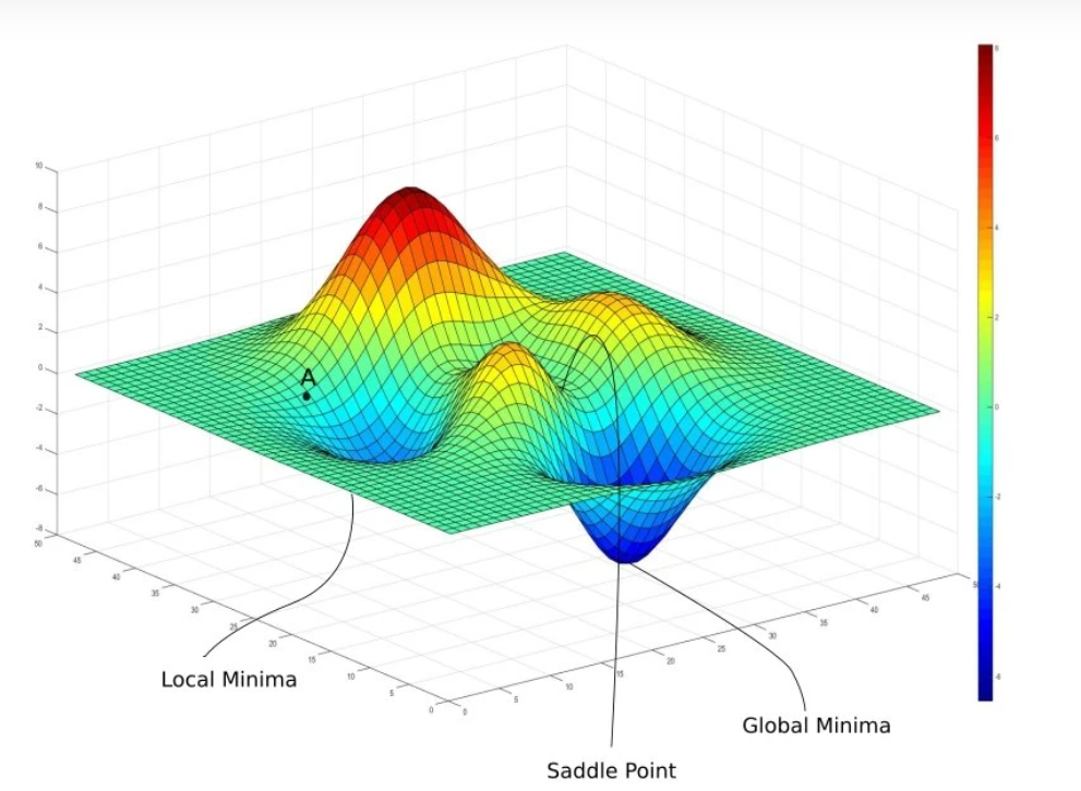
Set of weights for machine learning with a gradient descent method.
Gradient descent begins by selecting a random point within the space of weight. Our algorithm can only use local information from around this point because the rest of the space is unknown. Using the slope of the error surface at that location, the randomly selected weights can then be adjusted little by little in the direction of the error surface gradient to move to a new position on the error surface.
The adjustments are made in the direction of the error surface gradient, allowing for each new point to be slightly closer to the overall global minimum, until the global minimum is reached (where the slope is 0). The saddle point in the above image is the random point we start with. We then go to the local minimum and keep iterating the process until the global minimum is achieved.
Gradient Descent as an Algorithm (Batch Gradient Descent)
The gradient descent algorithm for training multivariable linear regression models requires a set of training instances (referred to as D), as well as a learning rate (α) for controlling the rate at which the algorithm converges, a convergence criterion that indicates when to stop the algorithm iterations, and lastly, an error delta function that determines the direction in which to adjust the randomized weight for coming closer to the global minimum.
Taking into consideration more than one variable changes the previous sum of squared errors for each training instance to:
Multivariable Sum of Squared Errors
Just as a reminder, D in this case refers to the set of training instances and w[j] (discussed later) is the randomly selected beginning weight.
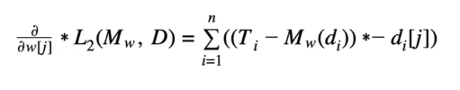
Error Delta Function for Multivariable Linear Regression
For each calculated gradient using the above equation for machine learning algorithms, we want to move in the opposite direction for the purpose of returning a lower value on the error surface. The error delta function calculates the delta value that determines the direction and the magnitude of the adjustments made to each weight.
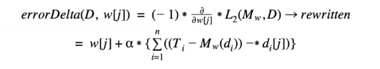
The delta value is determined by the gradient of the error surface at the latest position in the space of weight. Therefore, our error delta function (whose purpose is to calculate the direction to move in for a given weight), is:
The above is the weight update rule for multivariable linear regression with gradient descent, where tiis the expected target feature for i training instance and relates to w (the weight vector), di [j] (j^th descriptive feature corresponding to the i^th instance of training), and (the constant learning rate). The error delta function is the lower equation starting with the sigma sign (in curly brackets) within the greater weight update rule.
Error Delta Function
The above is the weight update rule for multivariable linear regression with gradient descent, where ti is the expected target feature for i training instance and relates to w (the weight vector), di [j] (j descriptive feature corresponding to the i instance of training), and (the constant learning rate). The error delta function is the lower equation starting with the sigma sign (in curly brackets) within the greater weight update rule.
Understanding the Weight Update Rule
Understanding the weight update rule for machine learning algorithms starts with understanding how it changes weights based on the error calculations by predictions made in the current candidate model.
If the errors show that predictions made by the model at hand are too high, then the weights should be decreased while di [j] is positive and increased while negative.
If the errors show that predictions made by the model at hand are too low, then the weights should be increased while di [j] is positive and increased while negative.
This process in its entirety is also known as “batch gradient descent” because one adjustment is made to each weight for each iteration, so the weights are changed in “batches.”
Logistic Regression
Logistic regression is useful when the dependent variable is “binary” in nature. This means logistic regression is usually associated with examining the association of independent variables with one dichotomous dependent variable. Meanwhile, linear regression is used for when the dependent variable is continuous, and the nature of the line of regression is linear.
A random example of how logistic regression has been used as an algorithm for machine learning is modeling how new words enter a language over time or how the amount of people using a product changes its buying patterns over time.
Logistic Regression Function
For logistic regression models, the output of the basic linear regression model is outputted using the logistic function. The logistic function is a threshold function that is continuous and differentiable.
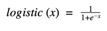
Logistic Function
For reference, the above equation represents e as Euler’s number (2.71828), the base of the natural logarithms, and x as the input value.
Instead of the regression function being the dot product of the weights and descriptive features like in linear and multivariable regression functions, the logistic function passes the dot products of weights and descriptive feature values through it. The decision surface that results from the above equation once values are substituted is quite different from the error surfaces we saw earlier for multivariable and linear regression.
Decision Surface for Logistic Regression
The decision surface for logistic regression is not to be confused with the error surfaces discussed earlier – they are two separate ideas. The decision surface shows the value of the logistic equation for every possible input value. Logistic regression usually has a gentle transition from faulty target predictions to good target predictions.
This is a benefit for using logistic regression, since the correct and incorrect prediction accuracies are not as “black and white” as they are for simple linear and multivariable regression. Logistic regression models can also be interpreted as probabilities of the occurrence of a target level (through the use of the logistic function).
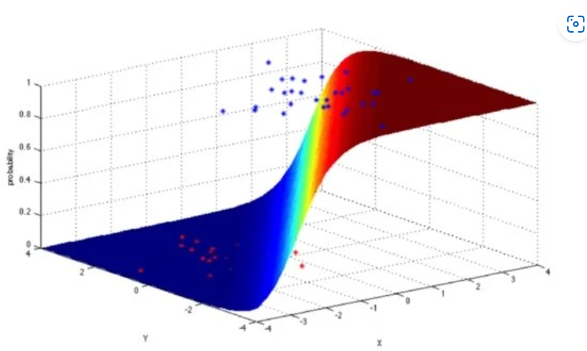
Decision Surface for Logistic Regression