Category: 10 Machine Learning Algorithms to Know in 2023

It is undeniably, machine learning and artificial intelligence have become immensely notorious over the past few years. Also, at the moment, big data is gaining notoriety in the tech industry where machine learning is amazingly powerful for delivering predictions or forecasting recommendations, relied on the huge amount of data. 

What are Machine Learning Algorithms?

Being a subset of Artificial Intelligence, Machine Learning is the technique that trains computers/systems to work independently, without being programmed explicitly.

And, during this process of training and learning, various algorithms come into the picture, that helps such systems in order to train themselves in a superior way with time, are referred as Machine Learning Algorithms. 

---

---

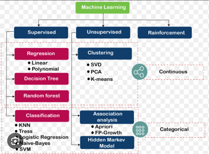
Machine learning algorithms work on the concept of three ubiquitous learning models:  supervised learning, unsupervised learning, and reinforcement learning. These are essentially the types of machine learning;

• Supervised learning is deployed in cases where a label data is available for specific datasets and identifies patterns within values labels assigned to data points. 
• Unsupervised learning is implemented in cases where the difficulty is to determine implicit connections in a given unlabeled dataset.
• Reinforcement learning selects an action, relied on each data point and after that learn how good the action was.

(Related blog: Fundamentals to Reinforcement Learning)

Machine Learning Algorithm

In the intense dynamic time, several machine learning algorithms have been developed in order to solve real-world problems; they are extremely automated and self-correcting as embracing the potential of improving over time while exploiting growing amounts of data and demanding minimal human intervention.

Let’s learn about some of the fascinating machine learning algorithms;

---

---

1. Decision Tree

The decision tree is the decision supporting tool that practices a tree-like graph or model of decisions along with their feasible outcomes, like the chance-event outcome, resource costs and implementation.

Being a supervised learning algorithm, decision trees are the best choice for classifying both categorical and continuous dependent variables. In this algorithm, the population is split into two or more homogeneous datasets, relying on the most significant characteristics or independent variables.

---

---

Over the graphical representation of the decision tree, the internal node highlights a test on the attribute, each individual branch denotes the outcome of the test, and leaf node signifies a specific class label, therefore the decision is made after computing all the attributes.

Fundamentally, decision trees are of two types;

• Classification Trees– Accounted as the default kind of decision trees, classification trees are adapted to distinct the dataset into various classes on the basis of the response variable, and preferred when the response variable is categorical in nature.
• Regression Trees– In opposite to the classification tree, regression trees are chosen when the response or target variable is continuous or numerical in nature and adapted in predictive based problems.

2. Naive Bayes Classifier

A Naive Bayes classifier believes that the appearance of a selective feature in a class is irrelevant to the appearance of any other feature. It considers all the properties independent while calculating the probability of a particular outcome, even if each feature are related to each other.

The model involves two types of probabilities 

• Probability of each class, and
• Conditional Probability for each class, given each x value.

Both the probabilities can be measured directly from training data, once calculated, the probability model can be deployed for making predictions for new data via Bayes Theorem.

Some of the real-world cases of naive Bayes classifiers are to label an email as spam or not, to categorize a new article in technology, politics or sports group, to identify a text stating positive or negative emotions, and in face and voice recognition software.

3. Ordinary Least Square Regression

Under statistics computation, Least Square is the method to perform linear regression. In order to establish the connection between a dependent variable and an independent variable, the ordinary least squares method is like- draw a straight line, later for each data point, calculate the vertical distance amidst the point and the line and summed these up.

---

---

The fitted line would be the one where the sum of distances is as small as possible. Least squares are referring to the sort of errors metric that are minimized.

4. Linear Regression

Linear Regression describes the impact on the dependent variable while the independent variable gets altered, as a consequence an independent variable is known as the explanatory variable whereas the dependent variable is named as the factor of interest.

It shows the connection amid an independent and a dependent variable and deals with prediction/estimations in continuous values. E.g. it can be used for risk assessment in the insurance domain, to identify the number of applications for multiple ages users.

The linear regression can be described in terms of a best fit relationship among the input variable (x) and output variable (y) through identifying the specific weights for the input variables, named as coefficients (B), that is

y= B₀ + B₁*x

---

---

5. Logistic Regression

Logistic regression is a powerful statistical tool of modelling a binomial outcome with one or more explanatory variables. It computes the association amid the categorical dependent variable and one or more independent variables through measuring probabilities by a logistic function (or cumulative logistics distribution). 

The Logistic Regression Algorithm works for discrete values, it is well suitable for binary classification where if an event occurs successfully, it is classified as 1, and 0, if not. Therefore, the probability of occurring of a specific event is estimated in the basis of provided predictor variables.

---

---

It has the real world applications as;

• Credit scoring 
• Estimating success rates of marketing campaigns
• Anticipating the revenues generated by a certain product or service.
• In politics, whether a particular candidate wins or loses the election. 

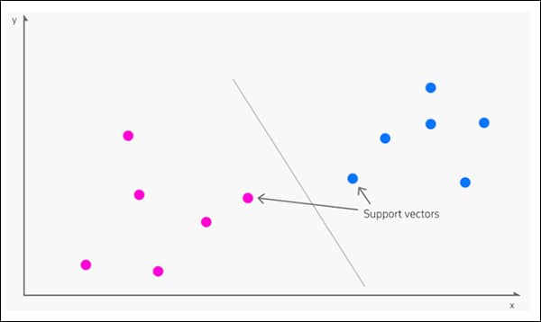
6. Support Vector Machines

In SVM, a hyperplane (a line that divides the input variable space) is selected to separate appropriately the data points across input variables space by their respective class either 0 or 1.

Basically, the SVM algorithm determines the coefficients that yield in the suitable separation of the various classes through the hyperplane, where the distance amid the hyperplane and the closest data points is referred to as the margin. However, the optimal hyperplane, that can depart the two classes, is the line that holds the largest margin.

---

---

Only such points are applicable in determining the hyperplane and the construction of the classifier and are termed as the support vectors as they support or define the hyperplane. 

More specifically, SVM renders appropriate classification for classification problems upon the training data, and extra efficiency for accurate classification of the future and also doesn’t overfit the data.

SVM is greatly used for stock market forecasting, for instance, one can use it to check the relative performance of the one stocks when compared to the other stocks under the same market. Thereby, with the help of the relative comparison of stocks, one can manage investment and make decisions depending upon the classifications made by SVM algorithm. 

7. Clustering Algorithms

Being an unsupervised learning problem, clustering approach is used as a data analysis technique for identifying informative data patterns, such as groups of customers based on their behavior or locations. Clustering descibes a class of problem and a class of methods, take a look at  Clustering Methods and Applications.

Clustering Algorithms refer to the group task of clustering, i.e. grouping an assemblage of objects in such a way that each object is more identical to each other under the same group (cluster) in comparison to those in separate groups.

There are various kinds of clustering algorithms that use similarity or distance measures amid examples in the feature space to find out dense regions of observations. Therefore, it is a good attempt to scale data previously for using clustering algorithms. However, each clustering algorithm is different, some of them are connectivity-based algorithms, dimensionality reduction, neural networks, probabilistic, etc. 

8. Gradient Boosting & AdaBoost

Boosting algorithms are used while dealing with massive quantities of data for making a prediction with great accuracy. It is an ensemble learning algorithm that integrates the predictive potential of diversified base estimators in order to enhance robustness, i.e. it blends the various vulnerable and mediocre predictors for developing strong predictor/estimator.

In simple terms, Boosting is the learning algorithm that makes an active classifier/predictor from a weak or average classifier. This process is achieved through creating a model from training data, and then constructing another second model in order to correct the errors from the first  model. Also, until the training set is precisely predicted, models are added or until the maximum number of models are joined.

These algorithms usually fit well in data science competitions like Kaggle, Hackathons, etc. As treated most preferred ML algorithms, these can be used with Python and R programming for obtaining accurate outcomes.

AdaBoost was the first competitive boosting algorithm that was constructed for binary classification. It can be considered as the initial step for learning and understanding boosting. Most of the modern boosting methods are constructed over AdaBoost, preferably on stochastic gradient boosting machines. 

The video below explains the AdaBoost which is just the simple twist on decision trees and random forests.

---

---

9. Principal Component Analysis

Dimensionality reduction algorithms are among the most important algorithms in machine learning that can be used when a data has multiple dimensions.

Consider a dataset that has “n” dimension, for instance a data professionlist is working on financial data that has the attributes as a credit score, personal details, personnel salary, etc. Now, in order to understand the important labels for building a required model, he/she can use dimensionality reduction method, and PCA is the appropriate algorithm for reducing dimensions.

PCA is a statistical approach that deploys an orthogonal transformation for reforming an array of observations of likely correlated variables into a set of observations of linearly uncorrelated variables, is known as principal components.

Using PCA, one can decrease the quantity of dimensions while retaining the important labels of the model. Since PCA is heavily relied on the number of dimensions, each PCA is perpendicular to the other and their dot product is zero.

---

---

Its applications include analysing data for smooth learning, and visualization. Since all the components of PCA have a very high variance, it is not an appropriate approach for noisy data.

10. Deep Learning Algorithms

Deep learning algorithms heavily rely on the nervous system of a human and are generally designed on the neural networks that use plentiful computational resources. All these algorithms use different types of neural networks to perform particular tasks.

They train computers by learning from examples and industries such as healthcare, eCommerce, entertainment, and advertising commonly use deep learning algorithms. 

Since, the deep learning algorithms signify self-learning representations, they basically coin ton ANNs that reflect the way a human brain functions and computes information. While the training process starts, algorithms intakes unknown components as the input data for extracting out features, group objects, and find out useful and hidden data patterns. 

These algorithms make use of several algorithms where no one single network is considered perfect and some algorithms are perfect fitted to perform specific tasks. However, in order to choose the correct ones, one should have a strong understanding of all primary algorithms

Some popular deep learning algorithms are Convolutional Neural Network (CNN), Recurrent Neural Networks (RNN), Long Short-Term Memory Networks (LSTM), etc.

Conclusion

From the above discussion, it can be concluded that Machine learning algorithms are programs/ models that learn from data and improve from experience regardless of the intervention of human being.

Google’s self-driving cars and robots get a lot of press, but the company’s real future is in machine learning, the technology that enables computers to get smarter and more personal. – Eric Schmidt (Google Chairman)

Some popular examples, where ML algorithms are being deployed, are Netflix’s algorithms that recommend movies based on the movies (or movie genre) we have watched in past, or Amazon’s algorithms that suggest an item, based on review or purchase history. 

Though we’re living through a time of extraordinary innovation in GPU-accelerated machine learning, the latest research papers frequently (and prominently) feature algorithms that are decades, in certain cases 70 years old.

Some might contend that many of these older methods fall into the camp of ‘statistical analysis’ rather than machine learning, and prefer to date the advent of the sector back only so far as 1957, with the invention of the Perceptron.

Given the extent to which these older algorithms support and are enmeshed in the latest trends and headline-grabbing developments in machine learning, it’s a contestable stance. So let’s take a look at some of the ‘classic’ building blocks underpinning the latest innovations, as well as some newer entries that are making an early bid for the AI hall of fame.

1: Transformers

In 2017 Google Research led a research collaboration culminating in the paper Attention Is All You Need. The work outlined a novel architecture that promoted attention mechanisms from ‘piping’ in encoder/decoder and recurrent network models to a central transformational technology in their own right.

The approach was dubbed Transformer, and has since become a revolutionary methodology in Natural Language Processing (NLP), powering, amongst many other examples, the autoregressive language model and AI poster-child GPT-3.

Transformers elegantly solved the problem of sequence transduction, also called ‘transformation’, which is occupied with the processing of input sequences into output sequences. A transformer also receives and manages data in a continuous manner, rather than in sequential batches, allowing a ‘persistence of memory’ which RNN architectures are not designed to obtain. For a more detailed overview of transformers, take a look at our reference article.

In contrast to the Recurrent Neural Networks (RNNs) that had begun to dominate ML research in the CUDA era, Transformer architecture could also be easily parallelized, opening the way to productively address a far larger corpus of data than RNNs.

Popular Usage

Transformers captured the public imagination in 2020 with the release of OpenAI’s GPT-3, which boasted a then record-breaking 175 billion parameters. This apparently staggering achievement was eventually overshadowed by later projects, such as the 2021 release of Microsoft’s Megatron-Turing NLG 530B, which (as the name suggests) features over 530 billion parameters.

A timeline of hyperscale Transformer NLP projects. Source: Microsoft

Transformer architecture has also crossed over from NLP to computer vision, powering a new generation of image synthesis frameworks such as OpenAI’s CLIP and DALL-E, which use text>image domain mapping to finish incomplete images and synthesize novel images from trained domains, among a growing number of related applications.

DALL-E attempts to complete a partial image of a bust of Plato. Source: https://openai.com/blog/dall-e/

2: Generative Adversarial Networks (GANs)

Though transformers have gained extraordinary media coverage through the release and adoption of GPT-3, the Generative Adversarial Network (GAN) has become a recognizable brand in its own right, and may eventually join deepfake as a verb.

First proposed in 2014 and primarily used for image synthesis, a Generative Adversarial Network architecture is composed of a Generator and a Discriminator. The Generator cycles through thousands of images in a dataset, iteratively attempting to reconstruct them. For each attempt, the Discriminator grades the Generator’s work, and sends the Generator back to do better, but without any insight into the way that the previous reconstruction erred.

Source: https://developers.google.com/machine-learning/gan/gan_structure

This forces the Generator to explore a multiplicity of avenues, instead of following the potential blind alleys that would have resulted if the Discriminator had told it where it was going wrong (see #8 below). By the time the training is over, the Generator has a detailed and comprehensive map of relationships between points in the dataset.

From the paper Improving GAN Equilibrium by Raising Spatial Awareness: a novel framework cycles through the sometimes-mysterious latent space of a GAN, providing responsive instrumentality for an image synthesis architecture. Source: https://genforce.github.io/eqgan/

By analogy, this is the difference between learning a single humdrum commute to central London, or painstakingly acquiring The Knowledge.

The result is a high-level collection of features in the latent space of the trained model. The semantic indicator for a high level feature could be ‘person’, whilst a descent through specificity related to the feature may unearth other learned characteristics, such as ‘male’ and ‘female’. At lower levels the sub-features can break down to, ‘blonde’, ‘Caucasian’, et al.

Entanglement is a notable issue in the latent space of GANs and encoder/decoder frameworks: is the smile on a GAN-generated female face an entangled feature of her ‘identity’ in the latent space, or is it a parallel branch?

GAN-generated faces from thispersondoesnotexist. Source: https://this-person-does-not-exist.com/en

The past couple of years have brought forth a growing number of new research initiatives in this respect, perhaps paving the way for feature-level, Photoshop-style editing for the latent space of a GAN, but at the moment, many transformations are effectively ‘all or nothing’ packages. Notably, NVIDIA’s EditGAN release of late 2021 achieves a high level of interpretability in the latent space by using semantic segmentation masks.

Popular Usage

Beside their (actually fairly limited) involvement in popular deepfake videos, image/video-centric GANs have proliferated over the last four years, enthralling researchers and the public alike. Keeping up with the dizzying rate and frequency of new releases is a challenge, though the GitHub repository Awesome GAN Applications aims to provide a comprehensive list.

Generative Adversarial Networks can in theory derive features from any well-framed domain, including text.

3: SVM

Originated in 1963, Support Vector Machine (SVM) is a core algorithm that crops up frequently in new research. Under SVM, vectors map the relative disposition of data points in a dataset, while support vectors delineate the boundaries between different groups, features, or traits.

Support vectors define the boundaries between groups. Source: https://www.kdnuggets.com/2016/07/support-vector-machines-simple-explanation.html

The derived boundary is called a hyperplane.

At low feature levels, the SVM is two-dimensional (image above), but where there’s a higher recognized number of groups or types, it becomes three-dimensional.

A deeper array of points and groups necessitates a three-dimensional SVM. Source: https://cml.rhul.ac.uk/svm.html

Popular Usage

Since support Vector Machines can effectively and agnostically address high-dimensional data of many kinds, they crop up widely across a variety of machine learning sectors, including deepfake detection, image classification, hate speech classification, DNA analysis and population structure prediction, among many others.

4: K-Means Clustering

Clustering in general is an unsupervised learning approach that seeks to categorize data points through density estimation, creating a map of the distribution of the data being studied.

K-Means clustering divines segments, groups and communities in data. Source: https://aws.amazon.com/blogs/machine-learning/k-means-clustering-with-amazon-sagemaker/

K-Means Clustering has become the most popular implementation of this approach, shepherding data points into distinctive ‘K Groups’, which may indicate demographic sectors, online communities, or any other possible secret aggregation waiting to be discovered in raw statistical data.

The K value itself is the determinant factor in the utility of the process, and in establishing an optimal value for a cluster. Initially, the K value is randomly assigned, and its features and vector characteristics compared to its neighbors. Those neighbors that most closely resemble the data point with the randomly assigned value get assigned to its cluster iteratively until the data has yielded all the groupings that the process permits.

The plot for the squared error, or ‘cost’ of differing values among the clusters will reveal an elbow point for the data:

The elbow point is similar in concept to the way that loss flattens out to diminishing returns at the end of a training session for a dataset. It represents the point at which no further distinctions between groups is going to become apparent, indicating the moment to move on to subsequent phases in the data pipeline, or else to report findings.

Popular Usage

K-Means Clustering, for obvious reasons, is a primary technology in customer analysis, since it offers a clear and explainable methodology to translate large quantities of commercial records into demographic insights and ‘leads’.

Outside of this application, K-Means Clustering is also employed for landslide prediction, medical image segmentation, image synthesis with GANs, document classification, and city planning, among many other potential and actual uses.

5: Random Forest

Random Forest is an ensemble learning method that averages the result from an array of decision trees to establish an overall prediction for the outcome.

If you’ve researched it even as little as watching the Back to the Future trilogy, a decision tree itself is fairly easy to conceptualize: a number of paths lie before you, and each path branches out to a new outcome which in turn contains further possible paths.

In reinforcement learning, you might retreat from a path and start again from an earlier stance, whereas decision trees commit to their journeys.

Thus the Random Forest algorithm is essentially spread-betting for decisions. The algorithm is called ‘random’ because it makes ad hoc selections and observations in order to understand the median sum of the results from the decision tree array.

Since it takes into account a multiplicity of factors, a Random Forest approach can be more difficult to convert into meaningful graphs than a decision tree, but is likely to be notably more productive.

Decision trees are subject to overfitting, where the results obtained are data-specific and not likely to generalize. Random Forest’s arbitrary selection of data points combats this tendency, drilling through to meaningful and useful representative trends in the data.

Popular Usage

As with many of the algorithms in this list, Random Forest typically operates as an ‘early’ sorter and filter of data, and as such consistently crops up in new research papers. Some examples of Random Forest usage include Magnetic Resonance Image Synthesis, Bitcoin price prediction, census segmentation, text classification and credit card fraud detection.

Since Random Forest is a low-level algorithm in machine learning architectures, it can also contribute to the performance of other low-level methods, as well as visualization algorithms, including Inductive Clustering, Feature Transformations, classification of text documents using sparse features, and displaying Pipelines.

6: Naive Bayes

Coupled with density estimation (see 4, above), a naive Bayes classifier is a powerful but relatively lightweight algorithm capable of estimating probabilities based on the calculated features of data.

The term ‘naïve’ refers to the assumption in Bayes’ theorem that features are unrelated, known as conditional independence. If you adopt this standpoint, walking and talking like a duck aren’t enough to establish that we’re dealing with a duck, and no ‘obvious’ assumptions are prematurely adopted.

This level of academic and investigative rigor would be overkill where ‘common sense’ is available, but is a valuable standard when traversing the many ambiguities and potentially unrelated correlations that may exist in a machine learning dataset.

In an original Bayesian network, features are subject to scoring functions, including minimal description length and Bayesian scoring, which can impose restrictions on the data in terms of the estimated connections found between the data points, and the direction in which these connections flow.

A naive Bayes classifier, conversely, operates by assuming that the features of a given object are independent, subsequently using Bayes’ theorem to calculate the probability of a given object, based on its features.

Popular Usage

Naive Bayes filters are well-represented in disease prediction and document categorization, spam filtering, sentiment classification, recommender systems, and fraud detection, among other applications.

7: K- Nearest Neighbors (KNN)

First proposed by the US Air Force School of Aviation Medicine in 1951, and having to accommodate itself to the state-of-the-art of mid-20th century computing hardware, K-Nearest Neighbors (KNN) is a lean algorithm that still features prominently across academic papers and private sector machine learning research initiatives.

KNN has been called ‘the lazy learner’, since it exhaustively scans a dataset in order to evaluate the relationships between data points, rather than requiring the training of a full-fledged machine learning model.

Though KNN is architecturally slender, its systematic approach does place a notable demand on read/write operations, and its use in very large datasets can be problematic without adjunct technologies such as Principal Component Analysis (PCA), which can transform complex and high volume datasets into representative groupings that KNN can traverse with less effort.

A recent study evaluated the effectiveness and economy of a number of algorithms tasked to predict whether an employee will leave a company, finding that the septuagenarian KNN remained superior to more modern contenders in terms of accuracy and predictive effectiveness.

Popular Usage

For all its popular simplicity of concept and execution, KNN is not stuck in the 1950s – it’s been adapted into a more DNN-focused approach in a 2018 proposal by Pennsylvania State University, and remains a central early-stage process (or post-processing analytical tool) in many far more complex machine learning frameworks.

In various configurations, KNN has been used or for online signature verification, image classification, text mining, crop prediction, and facial recognition, besides other applications and incorporations.

8: Markov Decision Process (MDP)

A mathematical framework introduced by American mathematician Richard Bellman in 1957, The Markov Decision Process (MDP) is one of the most basic blocks of reinforcement learning architectures. A conceptual algorithm in its own right, it has been adapted into a great number of other algorithms, and recurs frequently in the current crop of AI/ML research.

MDP explores a data environment by using its evaluation of its current state (i.e. ‘where’ it is in the data) to decide which node of the data to explore next.

A basic Markov Decision Process will prioritize near-term advantage over more desirable long-term objectives. For this reason, it is usually embedded into the context of a more comprehensive policy architecture in reinforcement learning, and is often subject to limiting factors such as discounted reward, and other modifying environmental variables that will prevent it from rushing to an immediate goal without consideration of the broader desired outcome.

Popular Usage

MDP’s low-level concept is widespread in both research and active deployments of machine learning. It’s been proposed for IoT security defense systems, fish harvesting, and market forecasting.

Besides its obvious applicability to chess and other strictly sequential games, MDP is also a natural contender for the procedural training of robotics systems, as we can see in the video below.

Global Planner using a Markov Decision Process – Mobile Industrial Robotics

9: Term Frequency-Inverse Document Frequency

Term Frequency (TF) divides the number of times a word appears in a document by the total number of words in that document. Thus the word seal appearing once in a thousand-word article has a term frequency of 0.001. By itself, TF is largely useless as an indicator of term importance, due to the fact that meaningless articles (such as a, and, the, and it) predominate.

To obtain a meaningful value for a term, Inverse Document Frequency (IDF) calculates the TF of a word across multiple documents in a dataset, assigning low rating to very high-frequency stopwords, such as articles. The resulting feature vectors are normalized to whole values, with each word assigned an appropriate weight.

TF-IDF weights the relevance of terms based on frequency across a number of documents, with rarer occurrence an indicator of salience. Source: https://moz.com/blog/inverse-document-frequency-and-the-importance-of-uniqueness

Though this approach prevents semantically important words from being lost as outliers, inverting the frequency weight does not automatically mean that a low-frequency term is not an outlier, because some things are rare and worthless. Therefore a low-frequency term will need to prove its value in the wider architectural context by featuring (even at a low frequency per document) in a number of documents in the dataset.

Despite its age, TF-IDF is a powerful and popular method for initial filtering passes in Natural Language Processing frameworks.

Popular Usage

Because TF-IDF has played at least some part in the development of Google’s largely occult PageRank algorithm over the last twenty years, it has become very widely adopted as a manipulative SEO tactic, in spite of John Mueller’s 2019 disavowal of its importance to search results.

Due to the secrecy around PageRank, there is no clear evidence that TF-IDF is not currently an effective tactic for rising in Google’s rankings. Incendiary discussion among IT professionals lately indicates a popular understanding, correct or not, that term abuse may still result in improved SEO placement (though additional accusations of monopoly abuse and excessive advertising blur the confines of this theory).

10: Stochastic Gradient Descent

Stochastic Gradient Descent (SGD) is an increasingly popular method for optimizing the training of machine learning models.

Gradient Descent itself is a method of optimizing and subsequently quantifying the improvement that a model is making during training.

In this sense, ‘gradient’ indicates a slope downwards (rather than a color-based gradation, see image below), where the highest point of the ‘hill’, on the left, represents the beginning of the training process. At this stage the model has not yet seen the entirety of the data even once, and has not learned enough about relationships between the data to produce effective transformations.

A gradient descent on a FaceSwap training session. We can see that the training has plateaued for some time in the second half, but has eventually recovered its way down the gradient towards an acceptable convergence.

The lowest point, on the right, represents convergence (the point at which the model is as effective as it is ever going to get under the imposed constraints and settings).

The gradient acts as a record and predictor for the disparity between the error rate (how accurately the model has currently mapped the data relationships) and the weights (the settings that influence the way in which the model will learn).

This record of progress can be used to inform a learning rate schedule, an automatic process that tells the architecture to become more granular and precise as the early vague details transform into clear relationships and mappings. In effect, gradient loss provides a just-in-time map of where the training should go next, and how it should proceed.

The innovation of Stochastic Gradient Descent is that it updates the model’s parameters on each training example per iteration, which generally speeds up the journey to convergence. Due to the advent of hyperscale datasets in recent years, SGD has grown in popularity lately as one possible method to address the ensuing logistic issues.

On the other hand, SGD has negative implications for feature scaling, and may require more iterations to achieve the same result, requiring additional planning and additional parameters, compared to regular Gradient Descent.

Popular Usage

Due to its configurability, and in spite of its shortcomings, SGD has become the most popular optimization algorithm for fitting neural networks. One configuration of SGD that is becoming dominant in new AI/ML research papers is the choice of the Adaptive Moment Estimation (ADAM, introduced in 2015) optimizer.

ADAM adapts the learning rate for each parameter dynamically (‘adaptive learning rate’), as well as incorporating results from previous updates into the subsequent configuration (‘momentum’). Additionally, it can be configured to use later innovations, such as Nesterov Momentum.

However, some maintain that the use of momentum can also speed ADAM (and similar algorithms) to a sub-optimal conclusion. As with most of the bleeding edge of the machine learning research sector, SGD is a work in progress.

Machine learning (ML) can do everything from analyzing X-rays to predicting stock market prices to recommending binge-worthy television shows. With such a wide range of applications, it’s not surprising that the global machine learning market is projected to grow from $21.7 billion in 2022 to $209.91 billion by 2029, according to Fortune Business Insights. 

At the core of machine learning are algorithms, which are trained to become the machine learning models used to power some of the most impactful innovations in the world today.

In this article, you’ll learn about 10 of the most popular machine learning algorithms that you’ll want to know, and explore the different learning styles used to turn machine learning algorithms into functioning machine learning models. 

10 machine learning algorithms to know

In simple terms, a machine learning algorithm is like a recipe that allows computers to learn and make predictions from data. Instead of explicitly telling the computer what to do, we provide it with a large amount of data and let it discover patterns, relationships, and insights on its own.

From classification to regression, here are 10 algorithms you need to know in the field of machine learning:

1. Linear regression

Linear regression is a supervised learning algorithm used for predicting and forecasting values that fall within a continuous range, such as sales numbers or housing prices. It is a technique derived from statistics and is commonly used to establish a relationship between an input variable (X) and an output variable (Y) that can be represented by a straight line.

In simple terms, linear regression takes a set of data points with known input and output values and finds the line that best fits those points. This line, known as the “regression line,” serves as a predictive model. By using this line, we can estimate or predict the output value (Y) for a given input value (X).

Linear regression is primarily used for predictive modeling rather than categorization. It is useful when we want to understand how changes in the input variable affect the output variable. By analyzing the slope and intercept of the regression line, we can gain insights into the relationship between the variables and make predictions based on this understanding.

2. Logistic regression

Logistic regression, also known as “logit regression,” is a supervised learning algorithm primarily used for binary classification tasks. It is commonly employed when we want to determine whether an input belongs to one class or another, such as deciding whether an image is a cat or not a cat. 

Logistic regression predicts the probability that an input can be categorized into a single primary class. However, in practice, it is commonly used to group outputs into two categories: the primary class and not the primary class. To accomplish this, logistic regression creates a threshold or boundary for binary classification. For example, any output value between 0 and 0.49 might be classified as one group, while values between 0.50 and 1.00 would be classified as the other group. 

Consequently, logistic regression is typically used for binary categorization rather than predictive modeling. It enables us to assign input data to one of two classes based on the probability estimate and a defined threshold. This makes logistic regression a powerful tool for tasks such as image recognition, spam email detection, or medical diagnosis where we need to categorize data into distinct classes.

3. Naive Bayes 

Naive Bayes is a set of supervised learning algorithms used to create predictive models for binary or multi-classification tasks. It is based on Bayes’ Theorem and operates on conditional probabilities, which estimate the likelihood of a classification based on the combined factors while assuming independence between them.

Let’s consider a program that identifies plants using a Naive Bayes algorithm. The algorithm takes into account specific factors such as perceived size, color, and shape to categorize images of plants. Although each of these factors is considered independently, the algorithm combines them to assess the probability of an object being a particular plant.

Naive Bayes leverages the assumption of independence among the factors, which simplifies the calculations and allows the algorithm to work efficiently with large datasets. It is particularly well-suited for tasks like document classification, email spam filtering, sentiment analysis, and many other applications where the factors can be considered separately but still contribute to the overall classification.

4. Decision tree

A decision tree is a supervised learning algorithm used for classification and predictive modeling tasks. It resembles a flowchart, starting with a root node that asks a specific question about the data. Based on the answer, the data is directed down different branches to subsequent internal nodes, which ask further questions and guide the data to subsequent branches. This process continues until the data reaches an end node, also known as a leaf node, where no further branching occurs.

Decision tree algorithms are popular in machine learning because they can handle complex datasets with ease and simplicity. The algorithm’s structure makes it straightforward to understand and interpret the decision-making process. By asking a sequence of questions and following the corresponding branches, decision trees enable us to classify or predict outcomes based on the data’s characteristics.

This simplicity and interpretability make decision trees valuable for various applications in machine learning, especially when dealing with complex datasets.

5. Random forest

A random forest algorithm is an ensemble of decision trees used for classification and predictive modeling. Instead of relying on a single decision tree, a random forest combines the predictions from multiple decision trees to make more accurate predictions.

In a random forest, numerous decision tree algorithms (sometimes hundreds or even thousands) are individually trained using different random samples from the training dataset. This sampling method is called “bagging.” Each decision tree is trained independently on its respective random sample.

Once trained, the random forest takes the same data and feeds it into each decision tree. Each tree produces a prediction, and the random forest tallies the results. The most common prediction among all the decision trees is then selected as the final prediction for the dataset.

Random forests address a common issue called “overfitting” that can occur with individual decision trees. Overfitting happens when a decision tree becomes too closely aligned with its training data, making it less accurate when presented with new data.

6. K-nearest neighbor (KNN)

K-nearest neighbor (KNN) is a supervised learning algorithm commonly used for classification and predictive modeling tasks. The name “K-nearest neighbor” reflects the algorithm’s approach of classifying an output based on its proximity to other data points on a graph. 

Let’s say we have a dataset with labeled points, some marked as blue and others as red. When we want to classify a new data point, KNN looks at its nearest neighbors in the graph. The “K” in KNN refers to the number of nearest neighbors considered. For example, if K is set to 5, the algorithm looks at the 5 closest points to the new data point.

Based on the majority of the labels among the K nearest neighbors, the algorithm assigns a classification to the new data point. For instance, if most of the nearest neighbors are blue points, the algorithm classifies the new point as belonging to the blue group.

Additionally, KNN can also be used for prediction tasks. Instead of assigning a class label, KNN can estimate the value of an unknown data point based on the average or median of its K nearest neighbors.

7.  K-means

K-means is an unsupervised learning algorithm commonly used for clustering and pattern recognition tasks. It aims to group data points based on their proximity to one another. Similar to K-nearest neighbor (KNN), K-means utilizes the concept of proximity to identify patterns or clusters in the data.

Each of the clusters is defined by a centroid, a real or imaginary center point for the cluster. K-means is useful on large data sets, especially for clustering, though it can falter when handling outliers.

K-means is particularly useful for large datasets and can provide insights into the inherent structure of the data by grouping similar points together. It has applications in various fields such as customer segmentation, image compression, and anomaly detection.

8. Support vector machine (SVM)

A support vector machine (SVM) is a supervised learning algorithm commonly used for classification and predictive modeling tasks. SVM algorithms are popular because they are reliable and can work well even with a small amount of data. SVM algorithms work by creating a decision boundary called a “hyperplane.” In two-dimensional space, this hyperplane is like a line that separates two sets of labeled data. 

The goal of SVM is to find the best possible decision boundary by maximizing the margin between the two sets of labeled data. It looks for the widest gap or space between the classes. Any new data point that falls on either side of this decision boundary is classified based on the labels in the training dataset.

It’s important to note that hyperplanes can take on different shapes when plotted in three-dimensional space, allowing SVM to handle more complex patterns and relationships in the data.

9. Apriori

Apriori is an unsupervised learning algorithm used for predictive modeling, particularly in the field of association rule mining. 

The Apriori algorithm was initially proposed in the early 1990s as a way to discover association rules between item sets. It is commonly used in pattern recognition and prediction tasks, such as understanding a consumer’s likelihood of purchasing one product after buying another.

The Apriori algorithm works by examining transactional data stored in a relational database. It identifies frequent itemsets, which are combinations of items that often occur together in transactions. These itemsets are then used to generate association rules. For example, if customers frequently buy product A and product B together, an association rule can be generated to suggest that purchasing A increases the likelihood of buying B.

By applying the Apriori algorithm, analysts can uncover valuable insights from transactional data, enabling them to make predictions or recommendations based on observed patterns of itemset associations.

10. Gradient boosting

Gradient boosting algorithms employ an ensemble method, which means they create a series of “weak” models that are iteratively improved upon to form a strong predictive model. The iterative process gradually reduces the errors made by the models, leading to the generation of an optimal and accurate final model.

The algorithm starts with a simple, naive model that may make basic assumptions, such as classifying data based on whether it is above or below the mean. This initial model serves as a starting point.

In each iteration, the algorithm builds a new model that focuses on correcting the mistakes made by the previous models. It identifies the patterns or relationships that the previous models struggled to capture and incorporates them into the new model.

Gradient boosting is effective in handling complex problems and large datasets. It can capture intricate patterns and dependencies that may be missed by a single model. By combining the predictions from multiple models, gradient boosting produces a powerful predictive model.

Get started in machine learning 

With Machine Learning from DeepLearning.AI on Coursera, you’ll have the opportunity to learn essential machine learning concepts and techniques from industry experts. Develop the skills to build and deploy machine learning models, analyze data, and make informed decisions through hands-on projects and interactive exercises. Not only will you build confidence in applying machine learning in various domains, you could also open doors to exciting career opportunities in data science.