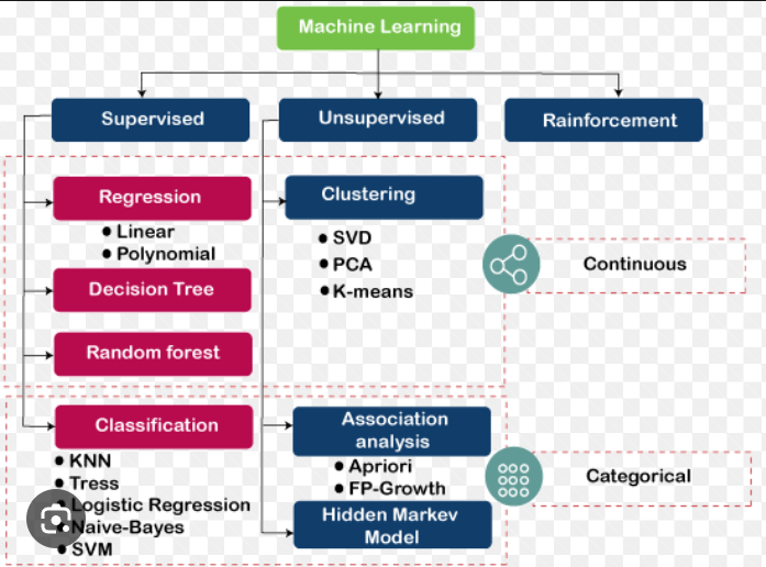
Supervised learning is an area of machine learning where the chosen algorithm tries to fit a target using the given input. A set of training data that contains labels is supplied to the algorithm. Based on a massive set of data, the algorithm will learn a rule that it uses to predict the labels for new observations. In other words, supervised learning algorithms are provided with historical data and asked to find the relationship that has the best predictive power.

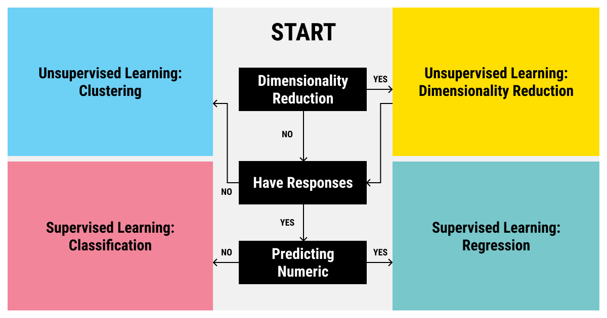
There are two varieties of supervised learning algorithms: regression and classification algorithms. Regression-based supervised learning methods try to predict outputs based on input variables. Classification-based supervised learning methods identify which category a set of data items belongs to. Classification algorithms are probability-based, meaning the outcome is the category for which the algorithm finds the highest probability that the dataset belongs to it. Regression algorithms, in contrast, estimate the outcome of problems that have an infinite number of solutions (continuous set of possible outcomes).

In the context of finance, supervised learning models represent one of the most-used class of machine learning models. Many algorithms that are widely applied in algorithmic trading rely on supervised learning models because they can be efficiently trained, they are relatively robust to noisy financial data, and they have strong links to the theory of finance.

Regression-based algorithms have been leveraged by academic and industry researchers to develop numerous asset pricing models. These models are used to predict returns over various time periods and to identify significant factors that drive asset returns. There are many other use cases of regression-based supervised learning in portfolio management and derivatives pricing.

Classification-based algorithms, on the other hand, have been leveraged across many areas within finance that require predicting a categorical response. These include fraud detection, default prediction, credit scoring, directional forecast of asset price movement, and Buy/Sell recommendations. There are many other use cases of classification-based supervised learning in portfolio management and algorithmic trading.

Many use cases of regression-based and classification-based supervised machine learning are presented in Chapters 5 and 6.

Python and its libraries provide methods and ways to implement these supervised learning models in few lines of code. Some of these libraries were covered in Chapter 2. With easy-to-use machine learning libraries like Scikit-learn and Keras, it is straightforward to fit different machine learning models on a given predictive modeling dataset.

In this chapter, we present a high-level overview of supervised learning models. For a thorough coverage of the topics, the reader is referred to Hands-On Machine Learning with Scikit-Learn, Keras, and TensorFlow, 2nd Edition, by Aurélien Géron (O’Reilly).

The following topics are covered in this chapter:

• Basic concepts of supervised learning models (both regression and classification).
• How to implement different supervised learning models in Python.
• How to tune the models and identify the optimal parameters of the models using grid search.
• Overfitting versus underfitting and bias versus variance.
• Strengths and weaknesses of several supervised learning models.
• How to use ensemble models, ANN, and deep learning models for both regression and classification.
• How to select a model on the basis of several factors, including model performance.
• Evaluation metrics for classification and regression models.
• How to perform cross validation.

Supervised Learning Models: An Overview

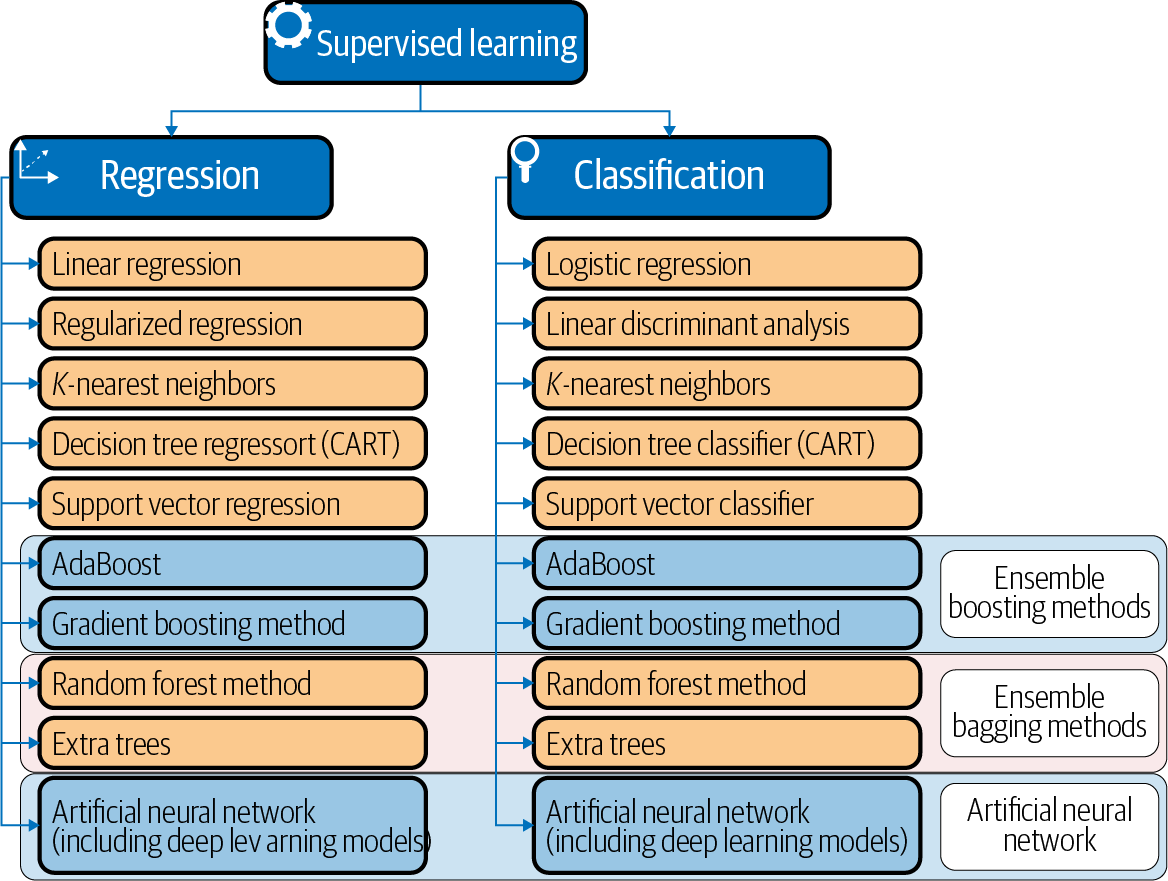
Classification predictive modeling problems are different from regression predictive modeling problems, as classification is the task of predicting a discrete class label and regression is the task of predicting a continuous quantity. However, both share the same concept of utilizing known variables to make predictions, and there is a significant overlap between the two models. Hence, the models for classification and regression are presented together in this chapter. Figure 4-1 summarizes the list of the models commonly used for classification and regression.

Some models can be used for both classification and regression with small modifications. These are K-nearest neighbors, decision trees, support vector, ensemble bagging/boosting methods, and ANNs (including deep neural networks), as shown in Figure 4-1. However, some models, such as linear regression and logistic regression, cannot (or cannot easily) be used for both problem types.

This section contains the following details about the models:

• Theory of the models.
• Implementation in Scikit-learn or Keras.
• Grid search for different models.
• Pros and cons of the models.

Note

In finance, a key focus is on models that extract signals from previously observed data in order to predict future values for the same time series. This family of time series models predicts continuous output and is more aligned with the supervised regression models. Time series models are covered separately in the supervised regression chapter (Chapter 5).

Linear Regression (Ordinary Least Squares)

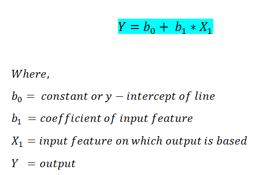
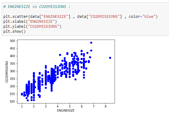
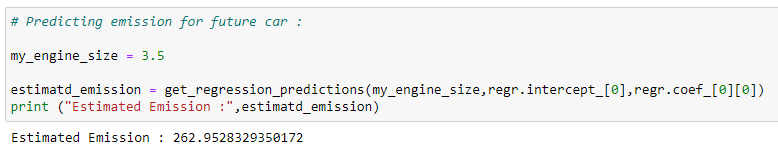
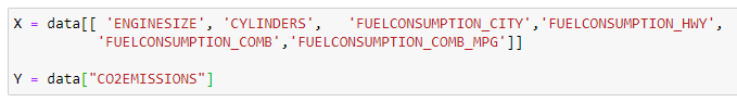
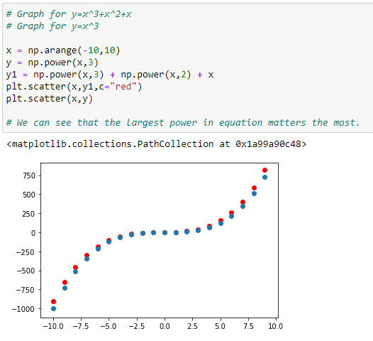
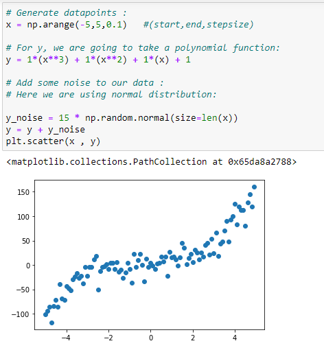
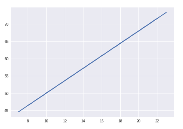
Linear regression (Ordinary Least Squares Regression or OLS Regression) is perhaps one of the most well-known and best-understood algorithms in statistics and machine learning. Linear regression is a linear model, e.g., a model that assumes a linear relationship between the input variables (x) and the single output variable (y). The goal of linear regression is to train a linear model to predict a new y given a previously unseen x with as little error as possible.

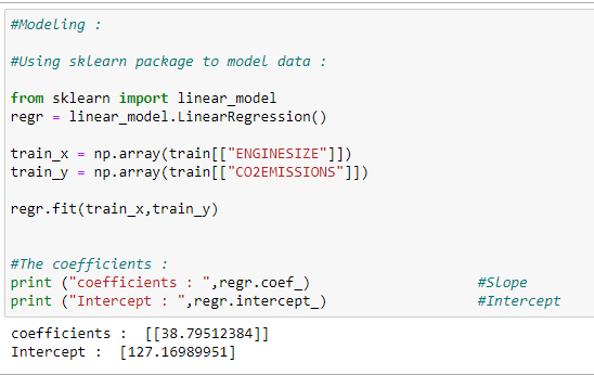
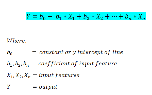
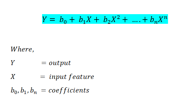
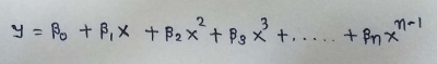
Our model will be a function that predicts y given �1,�2…��:�=�0+�1�1+…+����

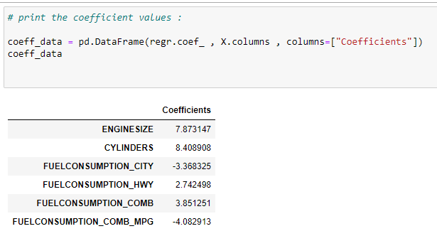
where, �0 is called intercept and �1…�� are the coefficient of the regression.

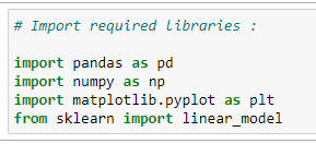
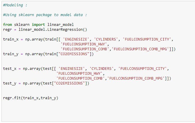
Implementation in Python

from sklearn.linear_model import LinearRegression
model = LinearRegression()
model.fit(X, Y)

In the following section, we cover the training of a linear regression model and grid search of the model. However, the overall concepts and related approaches are applicable to all other supervised learning models.

Training a model

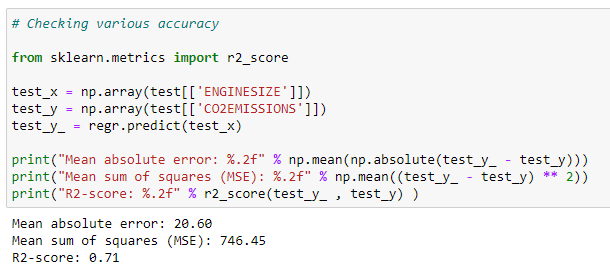
As we mentioned in Chapter 3, training a model basically means retrieving the model parameters by minimizing the cost (loss) function. The two steps for training a linear regression model are:Define a cost function (or loss function)

Measures how inaccurate the model’s predictions are. The sum of squared residuals (RSS) as defined in Equation 4-1 measures the squared sum of the difference between the actual and predicted value and is the cost function for linear regression.

Equation 4-1. Sum of squared residuals

���=∑�=1���–�0–∑�=1������2

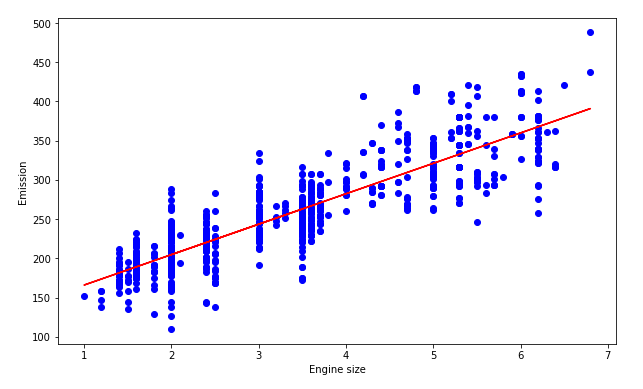
In this equation, �0 is the intercept; �� represents the coefficient; �1,..,�� are the coefficients of the regression; and ��� represents the ��ℎ observation and ��ℎ variable.Find the parameters that minimize loss

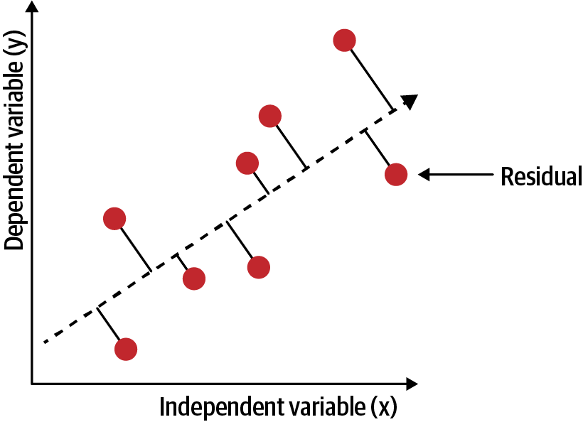
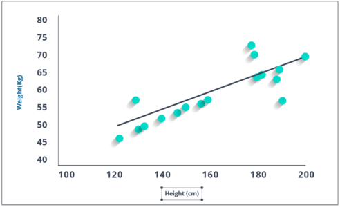
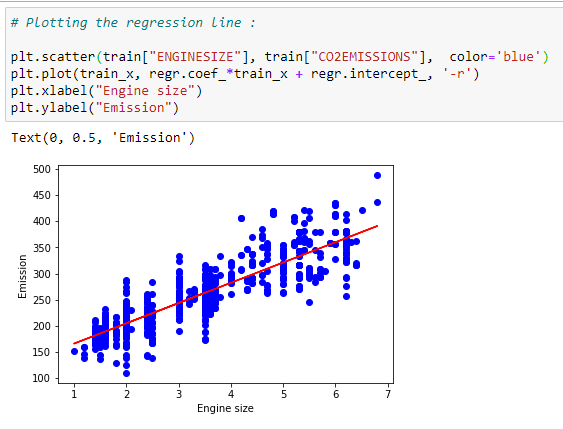
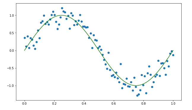
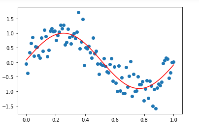
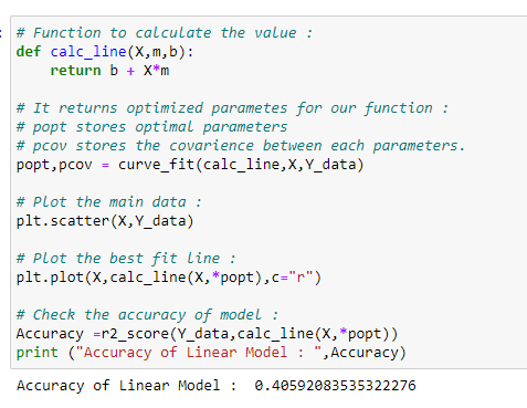
For example, make our model as accurate as possible. Graphically, in two dimensions, this results in a line of best fit as shown in Figure 4-2. In higher dimensions, we would have higher-dimensional hyperplanes. Mathematically, we look at the difference between each real data point (y) and our model’s prediction (ŷ). Square these differences to avoid negative numbers and penalize larger differences, and then add them up and take the average. This is a measure of how well our data fits the line.

Grid search

The overall idea of the grid search is to create a grid of all possible hyperparameter combinations and train the model using each one of them. Hyperparameters are the external characteristic of the model, can be considered the model’s settings, and are not estimated based on data-like model parameters. These hyperparameters are tuned during grid search to achieve better model performance.

Due to its exhaustive search, a grid search is guaranteed to find the optimal parameter within the grid. The drawback is that the size of the grid grows exponentially with the addition of more parameters or more considered values.

The GridSearchCV class in the model_selection module of the sklearn package facilitates the systematic evaluation of all combinations of the hyperparameter values that we would like to test.

The first step is to create a model object. We then define a dictionary where the keywords name the hyperparameters and the values list the parameter settings to be tested. For linear regression, the hyperparameter is fit_intercept, which is a boolean variable that determines whether or not to calculate the intercept for this model. If set to False, no intercept will be used in calculations:

model = LinearRegression()
param_grid = {'fit_intercept': [True, False]}
}

The second step is to instantiate the GridSearchCV object and provide the estimator object and parameter grid, as well as a scoring method and cross validation choice, to the initialization method. Cross validation is a resampling procedure used to evaluate machine learning models, and scoring parameter is the evaluation metrics of the model:¹

With all settings in place, we can fit GridSearchCV:

grid = GridSearchCV(estimator=model, param_grid=param_grid, scoring= 'r2', \
  cv=kfold)
grid_result = grid.fit(X, Y)

Advantages and disadvantages

In terms of advantages, linear regression is easy to understand and interpret. However, it may not work well when there is a nonlinear relationship between predicted and predictor variables. Linear regression is prone to overfitting (which we will discuss in the next section) and when a large number of features are present, it may not handle irrelevant features well. Linear regression also requires the data to follow certain assumptions, such as the absence of multicollinearity. If the assumptions fail, then we cannot trust the results obtained.

Regularized Regression

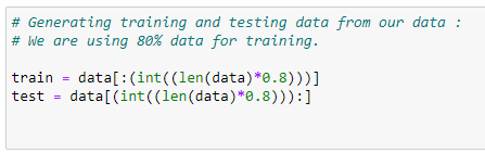
When a linear regression model contains many independent variables, their coefficients will be poorly determined, and the model will have a tendency to fit extremely well to the training data (data used to build the model) but fit poorly to testing data (data used to test how good the model is). This is known as overfitting or high variance.

One popular technique to control overfitting is regularization, which involves the addition of a penalty term to the error or loss function to discourage the coefficients from reaching large values. Regularization, in simple terms, is a penalty mechanism that applies shrinkage to model parameters (driving them closer to zero) in order to build a model with higher prediction accuracy and interpretation. Regularized regression has two advantages over linear regression:Prediction accuracy

The performance of the model working better on the testing data suggests that the model is trying to generalize from training data. A model with too many parameters might try to fit noise specific to the training data. By shrinking or setting some coefficients to zero, we trade off the ability to fit complex models (higher bias) for a more generalizable model (lower variance).Interpretation

A large number of predictors may complicate the interpretation or communication of the big picture of the results. It may be preferable to sacrifice some detail to limit the model to a smaller subset of parameters with the strongest effects.

The common ways to regularize a linear regression model are as follows:L1 regularization or Lasso regression

Lasso regression performs L1 regularization by adding a factor of the sum of the absolute value of coefficients in the cost function (RSS) for linear regression, as mentioned in Equation 4-1. The equation for lasso regularization can be represented as follows:

������������=���+�*∑�=1���

L1 regularization can lead to zero coefficients (i.e., some of the features are completely neglected for the evaluation of output). The larger the value of �, the more features are shrunk to zero. This can eliminate some features entirely and give us a subset of predictors, reducing model complexity. So Lasso regression not only helps in reducing overfitting, but also can help in feature selection. Predictors not shrunk toward zero signify that they are important, and thus L1 regularization allows for feature selection (sparse selection). The regularization parameter (�) can be controlled, and a lambda value of zero produces the basic linear regression equation.

A lasso regression model can be constructed using the Lasso class of the sklearn package of Python, as shown in the code snippet that follows:

from sklearn.linear_model import Lasso
model = Lasso()
model.fit(X, Y)

L2 regularization or Ridge regression

Ridge regression performs L2 regularization by adding a factor of the sum of the square of coefficients in the cost function (RSS) for linear regression, as mentioned in Equation 4-1. The equation for ridge regularization can be represented as follows:

������������=���+�*∑�=1���2

Ridge regression puts constraint on the coefficients. The penalty term (�) regularizes the coefficients such that if the coefficients take large values, the optimization function is penalized. So ridge regression shrinks the coefficients and helps to reduce the model complexity. Shrinking the coefficients leads to a lower variance and a lower error value. Therefore, ridge regression decreases the complexity of a model but does not reduce the number of variables; it just shrinks their effect. When � is closer to zero, the cost function becomes similar to the linear regression cost function. So the lower the constraint (low �) on the features, the more the model will resemble the linear regression model.

A ridge regression model can be constructed using the Ridge class of the sklearn package of Python, as shown in the code snippet that follows:

from sklearn.linear_model import Ridge
model = Ridge()
model.fit(X, Y)

Elastic net

Elastic nets add regularization terms to the model, which are a combination of both L1 and L2 regularization, as shown in the following equation:

������������=���+�*(1–�)/2*∑�=1���2+�*∑�=1���

In addition to setting and choosing a � value, an elastic net also allows us to tune the alpha parameter, where � = 0 corresponds to ridge and � = 1 to lasso. Therefore, we can choose an � value between 0 and 1 to optimize the elastic net. Effectively, this will shrink some coefficients and set some to 0 for sparse selection.

An elastic net regression model can be constructed using the ElasticNet class of the sklearn package of Python, as shown in the following code snippet:

from sklearn.linear_model import ElasticNet
model = ElasticNet()
model.fit(X, Y)

For all the regularized regression, � is the key parameter to tune during grid search in Python. In an elastic net, � can be an additional parameter to tune.

Logistic Regression

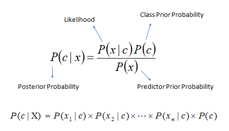
Logistic regression is one of the most widely used algorithms for classification. The logistic regression model arises from the desire to model the probabilities of the output classes given a function that is linear in x, at the same time ensuring that output probabilities sum up to one and remain between zero and one as we would expect from probabilities.

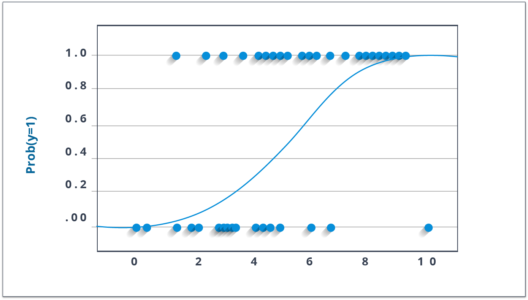
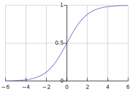
If we train a linear regression model on several examples where Y = 0 or 1, we might end up predicting some probabilities that are less than zero or greater than one, which doesn’t make sense. Instead, we use a logistic regression model (or logit model), which is a modification of linear regression that makes sure to output a probability between zero and one by applying the sigmoid function.²

Equation 4-2 shows the equation for a logistic regression model. Similar to linear regression, input values (x) are combined linearly using weights or coefficient values to predict an output value (y). The output coming from Equation 4-2 is a probability that is transformed into a binary value (0 or 1) to get the model prediction.

Equation 4-2. Logistic regression equation

�=exp(�0+�1�1+….+���1)1+exp(�0+�1�1+….+���1)

Where y is the predicted output, �0 is the bias or intercept term and B₁ is the coefficient for the single input value (x). Each column in the input data has an associated � coefficient (a constant real value) that must be learned from the training data.

In logistic regression, the cost function is basically a measure of how often we predicted one when the true answer was zero, or vice versa. Training the logistic regression coefficients is done using techniques such as maximum likelihood estimation (MLE) to predict values close to 1 for the default class and close to 0 for the other class.³

A logistic regression model can be constructed using the LogisticRegression class of the sklearn package of Python, as shown in the following code snippet:

from sklearn.linear_model import LogisticRegression
model = LogisticRegression()
model.fit(X, Y)

Hyperparameters

Regularization (penalty in sklearn)

Similar to linear regression, logistic regression can have regularization, which can be L1, L2, or elasticnet. The values in the sklearn library are [l1, l2, elasticnet].Regularization strength (C in sklearn)

This parameter controls the regularization strength. Good values of the penalty parameters can be [100, 10, 1.0, 0.1, 0.01].

Advantages and disadvantages

In terms of the advantages, the logistic regression model is easy to implement, has good interpretability, and performs very well on linearly separable classes. The output of the model is a probability, which provides more insight and can be used for ranking. The model has small number of hyperparameters. Although there may be risk of overfitting, this may be addressed using L1/L2 regularization, similar to the way we addressed overfitting for the linear regression models.

In terms of disadvantages, the model may overfit when provided with large numbers of features. Logistic regression can only learn linear functions and is less suitable to complex relationships between features and the target variable. Also, it may not handle irrelevant features well, especially if the features are strongly correlated.

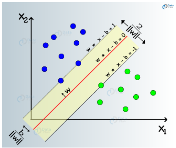
Support Vector Machine

The objective of the support vector machine (SVM) algorithm is to maximize the margin (shown as shaded area in Figure 4-3), which is defined as the distance between the separating hyperplane (or decision boundary) and the training samples that are closest to this hyperplane, the so-called support vectors. The margin is calculated as the perpendicular distance from the line to only the closest points, as shown in Figure 4-3. Hence, SVM calculates a maximum-margin boundary that leads to a homogeneous partition of all data points.

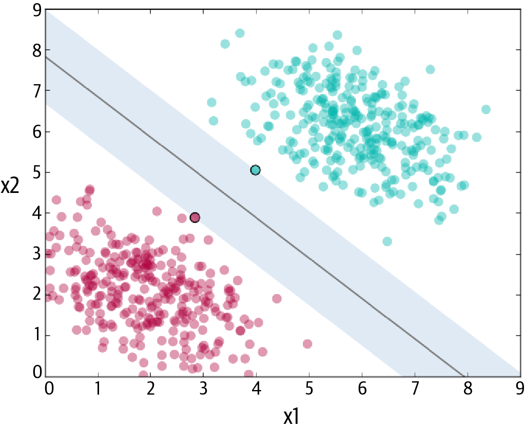
In practice, the data is messy and cannot be separated perfectly with a hyperplane. The constraint of maximizing the margin of the line that separates the classes must be relaxed. This change allows some points in the training data to violate the separating line. An additional set of coefficients is introduced that give the margin wiggle room in each dimension. A tuning parameter is introduced, simply called C, that defines the magnitude of the wiggle allowed across all dimensions. The larger the value of C, the more violations of the hyperplane are permitted.

In some cases, it is not possible to find a hyperplane or a linear decision boundary, and kernels are used. A kernel is just a transformation of the input data that allows the SVM algorithm to treat/process the data more easily. Using kernels, the original data is projected into a higher dimension to classify the data better.

SVM is used for both classification and regression. We achieve this by converting the original optimization problem into a dual problem. For regression, the trick is to reverse the objective. Instead of trying to fit the largest possible street between two classes while limiting margin violations, SVM regression tries to fit as many instances as possible on the street (shaded area in Figure 4-3) while limiting margin violations. The width of the street is controlled by a hyperparameter.

The SVM regression and classification models can be constructed using the sklearn package of Python, as shown in the following code snippets:

Regression

from sklearn.svm import SVR
model = SVR()
model.fit(X, Y)

Classification

from sklearn.svm import SVC
model = SVC()
model.fit(X, Y)

Hyperparameters

The following key parameters are present in the sklearn implementation of SVM and can be tweaked while performing the grid search:Kernels (kernel in sklearn)

The choice of kernel controls the manner in which the input variables will be projected. There are many kernels to choose from, but linear and RBF are the most common.Penalty (C in sklearn)

The penalty parameter tells the SVM optimization how much you want to avoid misclassifying each training example. For large values of the penalty parameter, the optimization will choose a smaller-margin hyperplane. Good values might be a log scale from 10 to 1,000.

Advantages and disadvantages

In terms of advantages, SVM is fairly robust against overfitting, especially in higher dimensional space. It handles the nonlinear relationships quite well, with many kernels to choose from. Also, there is no distributional requirement for the data.

In terms of disadvantages, SVM can be inefficient to train and memory-intensive to run and tune. It doesn’t perform well with large datasets. It requires the feature scaling of the data. There are also many hyperparameters, and their meanings are often not intuitive.

K-Nearest Neighbors

K-nearest neighbors (KNN) is considered a “lazy learner,” as there is no learning required in the model. For a new data point, predictions are made by searching through the entire training set for the K most similar instances (the neighbors) and summarizing the output variable for those K instances.

To determine which of the K instances in the training dataset are most similar to a new input, a distance measure is used. The most popular distance measure is Euclidean distance, which is calculated as the square root of the sum of the squared differences between a point a and a point b across all input attributes i, and which is represented as �(�,�)=∑�=1�(��–��)2. Euclidean distance is a good distance measure to use if the input variables are similar in type.

Another distance metric is Manhattan distance, in which the distance between point a and point b is represented as �(�,�)=∑�=1�|��–��|. Manhattan distance is a good measure to use if the input variables are not similar in type.

The steps of KNN can be summarized as follows:

1. Choose the number of K and a distance metric.
2. Find the K-nearest neighbors of the sample that we want to classify.
3. Assign the class label by majority vote.

KNN regression and classification models can be constructed using the sklearn package of Python, as shown in the following code:

Classification

from sklearn.neighbors import KNeighborsClassifier
model = KNeighborsClassifier()
model.fit(X, Y)

Regression

from sklearn.neighbors import KNeighborsRegressor
model = KNeighborsRegressor()
model.fit(X, Y)

Hyperparameters

The following key parameters are present in the sklearn implementation of KNN and can be tweaked while performing the grid search:Number of neighbors (n_neighbors in sklearn)

The most important hyperparameter for KNN is the number of neighbors (n_neighbors). Good values are between 1 and 20.Distance metric (metric in sklearn)

It may also be interesting to test different distance metrics for choosing the composition of the neighborhood. Good values are euclidean and manhattan.

Advantages and disadvantages

In terms of advantages, no training is involved and hence there is no learning phase. Since the algorithm requires no training before making predictions, new data can be added seamlessly without impacting the accuracy of the algorithm. It is intuitive and easy to understand. The model naturally handles multiclass classification and can learn complex decision boundaries. KNN is effective if the training data is large. It is also robust to noisy data, and there is no need to filter the outliers.

In terms of the disadvantages, the distance metric to choose is not obvious and difficult to justify in many cases. KNN performs poorly on high dimensional datasets. It is expensive and slow to predict new instances because the distance to all neighbors must be recalculated. KNN is sensitive to noise in the dataset. We need to manually input missing values and remove outliers. Also, feature scaling (standardization and normalization) is required before applying the KNN algorithm to any dataset; otherwise, KNN may generate wrong predictions.

Linear Discriminant Analysis

The objective of the linear discriminant analysis (LDA) algorithm is to project the data onto a lower-dimensional space in a way that the class separability is maximized and the variance within a class is minimized.⁴

During the training of the LDA model, the statistical properties (i.e., mean and covariance matrix) of each class are computed. The statistical properties are estimated on the basis of the following assumptions about the data:

• Data is normally distributed, so that each variable is shaped like a bell curve when plotted.
• Each attribute has the same variance, and the values of each variable vary around the mean by the same amount on average.

To make a prediction, LDA estimates the probability that a new set of inputs belongs to every class. The output class is the one that has the highest probability.

Implementation in Python and hyperparameters

The LDA classification model can be constructed using the sklearn package of Python, as shown in the following code snippet:

from sklearn.discriminant_analysis import LinearDiscriminantAnalysis
model = LinearDiscriminantAnalysis()
model.fit(X, Y)

The key hyperparameter for the LDA model is number of components for dimensionality reduction, which is represented by n_components in sklearn.

Advantages and disadvantages

In terms of advantages, LDA is a relatively simple model with fast implementation and is easy to implement. In terms of disadvantages, it requires feature scaling and involves complex matrix operations.

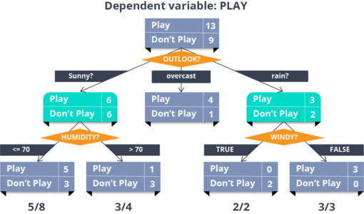
Classification and Regression Trees

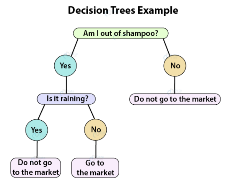
In the most general terms, the purpose of an analysis via tree-building algorithms is to determine a set of if–then logical (split) conditions that permit accurate prediction or classification of cases. Classification and regression trees (or CART or decision tree classifiers) are attractive models if we care about interpretability. We can think of this model as breaking down our data and making a decision based on asking a series of questions. This algorithm is the foundation of ensemble methods such as random forest and gradient boosting method.

Representation

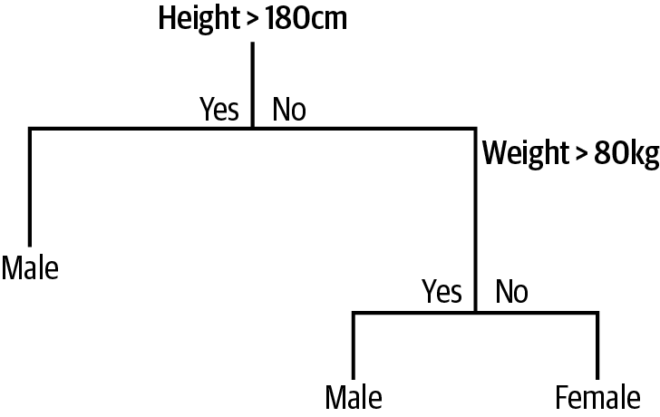
The model can be represented by a binary tree (or decision tree), where each node is an input variable x with a split point and each leaf contains an output variable y for prediction.

Figure 4-4 shows an example of a simple classification tree to predict whether a person is a male or a female based on two inputs of height (in centimeters) and weight (in kilograms).

Learning a CART model

Creating a binary tree is actually a process of dividing up the input space. A greedy approach called recursive binary splitting is used to divide the space. This is a numerical procedure in which all the values are lined up and different split points are tried and tested using a cost (loss) function. The split with the best cost (lowest cost, because we minimize cost) is selected. All input variables and all possible split points are evaluated and chosen in a greedy manner (e.g., the very best split point is chosen each time).

For regression predictive modeling problems, the cost function that is minimized to choose split points is the sum of squared errors across all training samples that fall within the rectangle:∑�=1�(��–�����������)2

where �� is the output for the training sample and prediction is the predicted output for the rectangle. For classification, the Gini cost function is used; it provides an indication of how pure the leaf nodes are (i.e., how mixed the training data assigned to each node is) and is defined as:�=∑�=1���*(1–��)

where G is the Gini cost over all classes and �� is the number of training instances with class k in the rectangle of interest. A node that has all classes of the same type (perfect class purity) will have G = 0, while a node that has a 50–50 split of classes for a binary classification problem (worst purity) will have G = 0.5.

Stopping criterion

The recursive binary splitting procedure described in the preceding section needs to know when to stop splitting as it works its way down the tree with the training data. The most common stopping procedure is to use a minimum count on the number of training instances assigned to each leaf node. If the count is less than some minimum, then the split is not accepted and the node is taken as a final leaf node.

Pruning the tree

The stopping criterion is important as it strongly influences the performance of the tree. Pruning can be used after learning the tree to further lift performance. The complexity of a decision tree is defined as the number of splits in the tree. Simpler trees are preferred as they are faster to run and easy to understand, consume less memory during processing and storage, and are less likely to overfit the data. The fastest and simplest pruning method is to work through each leaf node in the tree and evaluate the effect of removing it using a test set. A leaf node is removed only if doing so results in a drop in the overall cost function on the entire test set. The removal of nodes can be stopped when no further improvements can be made.

Implementation in Python

CART regression and classification models can be constructed using the sklearn package of Python, as shown in the following code snippet:

Classification

from sklearn.tree import DecisionTreeClassifier
model = DecisionTreeClassifier()
model.fit(X, Y)

Regression

from sklearn.tree import DecisionTreeRegressor
model = DecisionTreeRegressor ()
model.fit(X, Y)

Hyperparameters

CART has many hyperparameters. However, the key hyperparameter is the maximum depth of the tree model, which is the number of components for dimensionality reduction, and which is represented by max_depth in the sklearn package. Good values can range from 2 to 30 depending on the number of features in the data.

Advantages and disadvantages

In terms of advantages, CART is easy to interpret and can adapt to learn complex relationships. It requires little data preparation, and data typically does not need to be scaled. Feature importance is built in due to the way decision nodes are built. It performs well on large datasets. It works for both regression and classification problems.

In terms of disadvantages, CART is prone to overfitting unless pruning is used. It can be very nonrobust, meaning that small changes in the training dataset can lead to quite major differences in the hypothesis function that gets learned. CART generally has worse performance than ensemble models, which are covered next.

Ensemble Models

The goal of ensemble models is to combine different classifiers into a meta-classifier that has better generalization performance than each individual classifier alone. For example, assuming that we collected predictions from 10 experts, ensemble methods would allow us to strategically combine their predictions to come up with a prediction that is more accurate and robust than the experts’ individual predictions.

The two most popular ensemble methods are bagging and boosting. Bagging (or bootstrap aggregation) is an ensemble technique of training several individual models in a parallel way. Each model is trained by a random subset of the data. Boosting, on the other hand, is an ensemble technique of training several individual models in a sequential way. This is done by building a model from the training data and then creating a second model that attempts to correct the errors of the first model. Models are added until the training set is predicted perfectly or a maximum number of models is added. Each individual model learns from mistakes made by the previous model. Just like the decision trees themselves, bagging and boosting can be used for classification and regression problems.

By combining individual models, the ensemble model tends to be more flexible (less bias) and less data-sensitive (less variance).⁵ Ensemble methods combine multiple, simpler algorithms to obtain better performance.

In this section we will cover random forest, AdaBoost, the gradient boosting method, and extra trees, along with their implementation using sklearn package.

Random forest

Random forest is a tweaked version of bagged decision trees. In order to understand a random forest algorithm, let us first understand the bagging algorithm. Assuming we have a dataset of one thousand instances, the steps of bagging are:

1. Create many (e.g., one hundred) random subsamples of our dataset.
2. Train a CART model on each sample.
3. Given a new dataset, calculate the average prediction from each model and aggregate the prediction by each tree to assign the final label by majority vote.

A problem with decision trees like CART is that they are greedy. They choose the variable to split by using a greedy algorithm that minimizes error. Even after bagging, the decision trees can have a lot of structural similarities and result in high correlation in their predictions. Combining predictions from multiple models in ensembles works better if the predictions from the submodels are uncorrelated, or at best are weakly correlated. Random forest changes the learning algorithm in such a way that the resulting predictions from all of the subtrees have less correlation.

In CART, when selecting a split point, the learning algorithm is allowed to look through all variables and all variable values in order to select the most optimal split point. The random forest algorithm changes this procedure such that each subtree can access only a random sample of features when selecting the split points. The number of features that can be searched at each split point (m) must be specified as a parameter to the algorithm.

As the bagged decision trees are constructed, we can calculate how much the error function drops for a variable at each split point. In regression problems, this may be the drop in sum squared error, and in classification, this might be the Gini cost. The bagged method can provide feature importance by calculating and averaging the error function drop for individual variables.

Implementation in Python

Random forest regression and classification models can be constructed using the sklearn package of Python, as shown in the following code:

Classification

from sklearn.ensemble import RandomForestClassifier
model = RandomForestClassifier()
model.fit(X, Y)

Regression

from sklearn.ensemble import RandomForestRegressor
model = RandomForestRegressor()
model.fit(X, Y)

Hyperparameters

Some of the main hyperparameters that are present in the sklearn implementation of random forest and that can be tweaked while performing the grid search are:Maximum number of features (max_features in sklearn)

This is the most important parameter. It is the number of random features to sample at each split point. You could try a range of integer values, such as 1 to 20, or 1 to half the number of input features.Number of estimators (n_estimators in sklearn)

This parameter represents the number of trees. Ideally, this should be increased until no further improvement is seen in the model. Good values might be a log scale from 10 to 1,000.

Advantages and disadvantages

The random forest algorithm (or model) has gained huge popularity in ML applications during the last decade due to its good performance, scalability, and ease of use. It is flexible and naturally assigns feature importance scores, so it can handle redundant feature columns. It scales to large datasets and is generally robust to overfitting. The algorithm doesn’t need the data to be scaled and can model a nonlinear relationship.

In terms of disadvantages, random forest can feel like a black box approach, as we have very little control over what the model does, and the results may be difficult to interpret. Although random forest does a good job at classification, it may not be good for regression problems, as it does not give a precise continuous nature prediction. In the case of regression, it doesn’t predict beyond the range in the training data and may overfit datasets that are particularly noisy.

Extra trees

Extra trees, otherwise known as extremely randomized trees, is a variant of a random forest; it builds multiple trees and splits nodes using random subsets of features similar to random forest. However, unlike random forest, where observations are drawn with replacement, the observations are drawn without replacement in extra trees. So there is no repetition of observations.

Additionally, random forest selects the best split to convert the parent into the two most homogeneous child nodes.⁶ However, extra trees selects a random split to divide the parent node into two random child nodes. In extra trees, randomness doesn’t come from bootstrapping the data; it comes from the random splits of all observations.

In real-world cases, performance is comparable to an ordinary random forest, sometimes a bit better. The advantages and disadvantages of extra trees are similar to those of random forest.

Implementation in Python

Extra trees regression and classification models can be constructed using the sklearn package of Python, as shown in the following code snippet. The hyperparameters of extra trees are similar to random forest, as shown in the previous section:

Classification

from sklearn.ensemble import ExtraTreesClassifier
model = ExtraTreesClassifier()
model.fit(X, Y)

Regression

from sklearn.ensemble import ExtraTreesRegressor
model = ExtraTreesRegressor()
model.fit(X, Y)

Adaptive Boosting (AdaBoost)

Adaptive Boosting or AdaBoost is a boosting technique in which the basic idea is to try predictors sequentially, and each subsequent model attempts to fix the errors of its predecessor. At each iteration, the AdaBoost algorithm changes the sample distribution by modifying the weights attached to each of the instances. It increases the weights of the wrongly predicted instances and decreases the ones of the correctly predicted instances.

The steps of the AdaBoost algorithm are:

1. Initially, all observations are given equal weights.
2. A model is built on a subset of data, and using this model, predictions are made on the whole dataset. Errors are calculated by comparing the predictions and actual values.
3. While creating the next model, higher weights are given to the data points that were predicted incorrectly. Weights can be determined using the error value. For instance, the higher the error, the more weight is assigned to the observation.
4. This process is repeated until the error function does not change, or until the maximum limit of the number of estimators is reached.

Implementation in Python

AdaBoost regression and classification models can be constructed using the sklearn package of Python, as shown in the following code snippet:

Classification

from sklearn.ensemble import AdaBoostClassifier
model = AdaBoostClassifier()
model.fit(X, Y)

Regression

from sklearn.ensemble import AdaBoostRegressor
model = AdaBoostRegressor()
model.fit(X, Y)

Hyperparameters

Some of the main hyperparameters that are present in the sklearn implementation of AdaBoost and that can be tweaked while performing the grid search are as follows:Learning rate (learning_rate in sklearn)

Learning rate shrinks the contribution of each classifier/regressor. It can be considered on a log scale. The sample values for grid search can be 0.001, 0.01, and 0.1.Number of estimators (n_estimators in sklearn)

This parameter represents the number of trees. Ideally, this should be increased until no further improvement is seen in the model. Good values might be a log scale from 10 to 1,000.

Advantages and disadvantages

In terms of advantages, AdaBoost has a high degree of precision. AdaBoost can achieve similar results to other models with much less tweaking of parameters or settings. The algorithm doesn’t need the data to be scaled and can model a nonlinear relationship.

In terms of disadvantages, the training of AdaBoost is time consuming. AdaBoost can be sensitive to noisy data and outliers, and data imbalance leads to a decrease in classification accuracy

Gradient boosting method

Gradient boosting method (GBM) is another boosting technique similar to AdaBoost, where the general idea is to try predictors sequentially. Gradient boosting works by sequentially adding the previous underfitted predictions to the ensemble, ensuring the errors made previously are corrected.

The following are the steps of the gradient boosting algorithm:

1. A model (which can be referred to as the first weak learner) is built on a subset of data. Using this model, predictions are made on the whole dataset.
2. Errors are calculated by comparing the predictions and actual values, and the loss is calculated using the loss function.
3. A new model is created using the errors of the previous step as the target variable. The objective is to find the best split in the data to minimize the error. The predictions made by this new model are combined with the predictions of the previous. New errors are calculated using this predicted value and actual value.
4. This process is repeated until the error function does not change or until the maximum limit of the number of estimators is reached.

Contrary to AdaBoost, which tweaks the instance weights at every interaction, this method tries to fit the new predictor to the residual errors made by the previous predictor.

Implementation in Python and hyperparameters

Gradient boosting method regression and classification models can be constructed using the sklearn package of Python, as shown in the following code snippet. The hyperparameters of gradient boosting method are similar to AdaBoost, as shown in the previous section:

Classification

from sklearn.ensemble import GradientBoostingClassifier
model = GradientBoostingClassifier()
model.fit(X, Y)

Regression

from sklearn.ensemble import GradientBoostingRegressor
model = GradientBoostingRegressor()
model.fit(X, Y)

Advantages and disadvantages

In terms of advantages, gradient boosting method is robust to missing data, highly correlated features, and irrelevant features in the same way as random forest. It naturally assigns feature importance scores, with slightly better performance than random forest. The algorithm doesn’t need the data to be scaled and can model a nonlinear relationship.

In terms of disadvantages, it may be more prone to overfitting than random forest, as the main purpose of the boosting approach is to reduce bias and not variance. It has many hyperparameters to tune, so model development may not be as fast. Also, feature importance may not be robust to variation in the training dataset.

ANN-Based Models

In Chapter 3 we covered the basics of ANNs, along with the architecture of ANNs and their training and implementation in Python. The details provided in that chapter are applicable across all areas of machine learning, including supervised learning. However, there are a few additional details from the supervised learning perspective, which we will cover in this section.

Neural networks are reducible to a classification or regression model with the activation function of the node in the output layer. In the case of a regression problem, the output node has linear activation function (or no activation function). A linear function produces a continuous output ranging from -inf to +inf. Hence, the output layer will be the linear function of the nodes in the layer before the output layer, and it will be a regression-based model.

In the case of a classification problem, the output node has a sigmoid or softmax activation function. A sigmoid or softmax function produces an output ranging from zero to one to represent the probability of target value. Softmax function can also be used for multiple groups for classification.

ANN using sklearn

ANN regression and classification models can be constructed using the sklearn package of Python, as shown in the following code snippet:

Classification

from sklearn.neural_network import MLPClassifier
model = MLPClassifier()
model.fit(X, Y)

Regression

from sklearn.neural_network import MLPRegressor
model = MLPRegressor()
model.fit(X, Y)

Hyperparameters

As we saw in Chapter 3, ANN has many hyperparameters. Some of the hyperparameters that are present in the sklearn implementation of ANN and can be tweaked while performing the grid search are:Hidden Layers (hidden_layer_sizes in sklearn)

It represents the number of layers and nodes in the ANN architecture. In sklearn implementation of ANN, the ith element represents the number of neurons in the ith hidden layer. A sample value for grid search in the sklearn implementation can be [(20,), (50,), (20, 20), (20, 30, 20)].Activation Function (activation in sklearn)

It represents the activation function of a hidden layer. Some of the activation functions defined in Chapter 3, such as sigmoid, relu, or tanh, can be used.

Deep neural network

ANNs with more than a single hidden layer are often called deep networks. We prefer using the library Keras to implement such networks, given the flexibility of the library. The detailed implementation of a deep neural network in Keras was shown in Chapter 3. Similar to MLPClassifier and MLPRegressor in sklearn for classification and regression, Keras has modules called KerasClassifier and KerasRegressor that can be used for creating classification and regression models with deep network.

A popular problem in finance is time series prediction, which is predicting the next value of a time series based on a historical overview. Some of the deep neural networks, such as recurrent neural network (RNN), can be directly used for time series prediction. The details of this approach are provided in Chapter 5.

Advantages and disadvantages

The main advantage of an ANN is that it captures the nonlinear relationship between the variables quite well. ANN can more easily learn rich representations and is good with a large number of input features with a large dataset. ANN is flexible in how it can be used. This is evident from its use across a wide variety of areas in machine learning and AI, including reinforcement learning and NLP, as discussed in Chapter 3.

The main disadvantage of ANN is the interpretability of the model, which is a drawback that often cannot be ignored and is sometimes the determining factor when choosing a model. ANN is not good with small datasets and requires a lot of tweaking and guesswork. Choosing the right topology/algorithms to solve a problem is difficult. Also, ANN is computationally expensive and can take a lot of time to train.

Using ANNs for supervised learning in finance

If a simple model such as linear or logistic regression perfectly fits your problem, don’t bother with ANN. However, if you are modeling a complex dataset and feel a need for better prediction power, give ANN a try. ANN is one of the most flexible models in adapting itself to the shape of the data, and using it for supervised learning problems can be an interesting and valuable exercise.

Model Performance

In the previous section, we discussed grid search as a way to find the right hyperparameter to achieve better performance. In this section, we will expand on that process by discussing the key components of evaluating the model performance, which are overfitting, cross validation, and evaluation metrics.

Overfitting and Underfitting

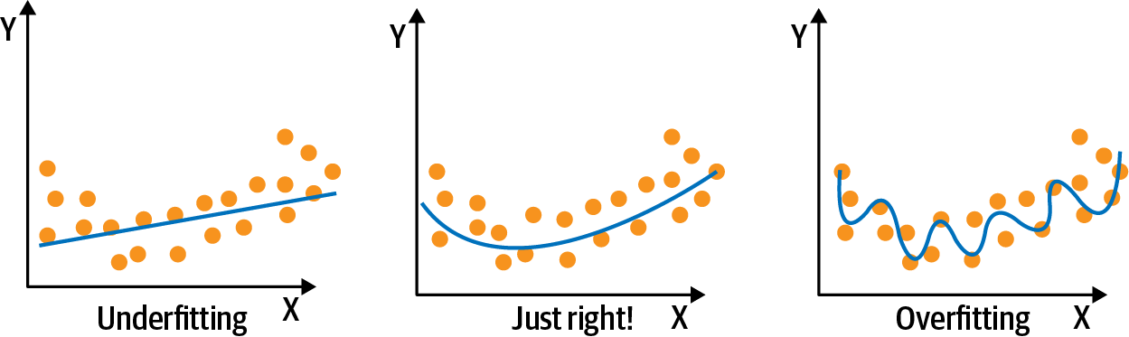
A common problem in machine learning is overfitting, which is defined by learning a function that perfectly explains the training data that the model learned from but doesn’t generalize well to unseen test data. Overfitting happens when a model overlearns from the training data to the point that it starts picking up idiosyncrasies that aren’t representative of patterns in the real world. This becomes especially problematic as we make our models increasingly more complex. Underfitting is a related issue in which the model is not complex enough to capture the underlying trend in the data. Figure 4-5 illustrates overfitting and underfitting. The left-hand panel of Figure 4-5 shows a linear regression model; a straight line clearly underfits the true function. The middle panel shows that a high degree polynomial approximates the true relationship reasonably well. On the other hand, a polynomial of a very high degree fits the small sample almost perfectly, and performs best on the training data, but this doesn’t generalize, and it would do a horrible job at explaining a new data point.

The concepts of overfitting and underfitting are closely linked to bias-variance trade-off. Bias refers to the error due to overly simplistic assumptions or faulty assumptions in the learning algorithm. Bias results in underfitting of the data, as shown in the left-hand panel of Figure 4-5. A high bias means our learning algorithm is missing important trends among the features. Variance refers to the error due to an overly complex model that tries to fit the training data as closely as possible. In high variance cases, the model’s predicted values are extremely close to the actual values from the training set. High variance gives rise to overfitting, as shown in the right-hand panel of Figure 4-5. Ultimately, in order to have a good model, we need low bias and low variance.

There can be two ways to combat overfitting:Using more training data

The more training data we have, the harder it is to overfit the data by learning too much from any single training example.Using regularization

Adding a penalty in the loss function for building a model that assigns too much explanatory power to any one feature, or allows too many features to be taken into account.

The concept of overfitting and the ways to combat it are applicable across all the supervised learning models. For example, regularized regressions address overfitting in linear regression, as discussed earlier in this chapter.

Cross Validation

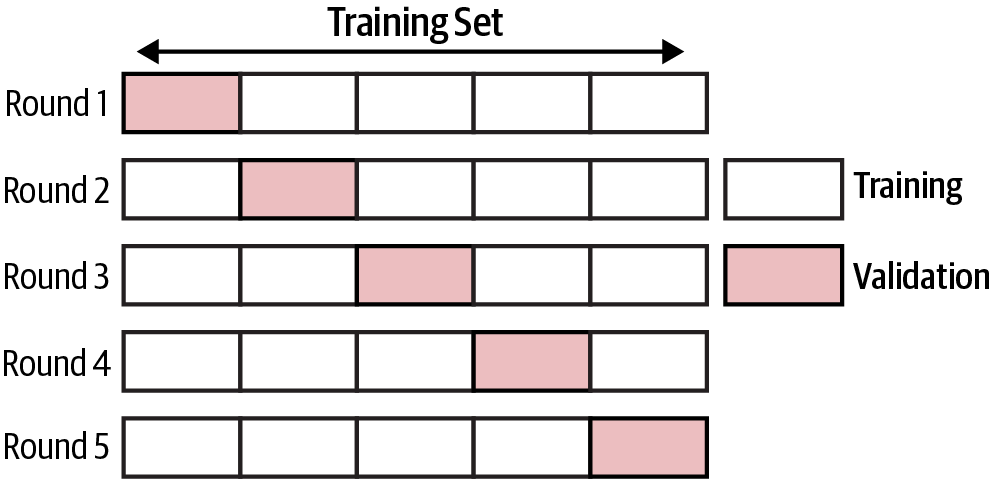
One of the challenges of machine learning is training models that are able to generalize well to unseen data (overfitting versus underfitting or a bias-variance trade-off). The main idea behind cross validation is to split the data one time or several times so that each split is used once as a validation set and the remainder is used as a training set: part of the data (the training sample) is used to train the algorithm, and the remaining part (the validation sample) is used for estimating the risk of the algorithm. Cross validation allows us to obtain reliable estimates of the model’s generalization error. It is easiest to understand it with an example. When doing k-fold cross validation, we randomly split the training data into k folds. Then we train the model using k-1 folds and evaluate the performance on the kth fold. We repeat this process k times and average the resulting scores.

Figure 4-6 shows an example of cross validation, where the data is split into five sets and in each round one of the sets is used for validation.

A potential drawback of cross validation is the computational cost, especially when paired with a grid search for hyperparameter tuning. Cross validation can be performed in a couple of lines using the sklearn package; we will perform cross validation in the supervised learning case studies.

In the next section, we cover the evaluation metrics for the supervised learning models that are used to measure and compare the models’ performance.

Evaluation Metrics

The metrics used to evaluate the machine learning algorithms are very important. The choice of metrics to use influences how the performance of machine learning algorithms is measured and compared. The metrics influence both how you weight the importance of different characteristics in the results and your ultimate choice of algorithm.

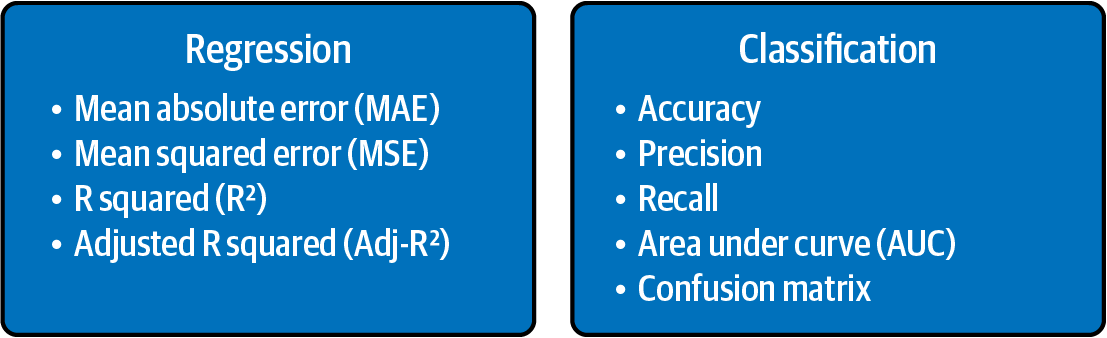
The main evaluation metrics for regression and classification are illustrated in Figure 4-7.

Let us first look at the evaluation metrics for supervised regression.

Mean absolute error

The mean absolute error (MAE) is the sum of the absolute differences between predictions and actual values. The MAE is a linear score, which means that all the individual differences are weighted equally in the average. It gives an idea of how wrong the predictions were. The measure gives an idea of the magnitude of the error, but no idea of the direction (e.g., over- or underpredicting).

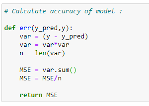
Mean squared error

The mean squared error (MSE) represents the sample standard deviation of the differences between predicted values and observed values (called residuals). This is much like the mean absolute error in that it provides a gross idea of the magnitude of the error. Taking the square root of the mean squared error converts the units back to the original units of the output variable and can be meaningful for description and presentation. This is called the root mean squared error (RMSE).

R² metric

The R² metric provides an indication of the “goodness of fit” of the predictions to actual value. In statistical literature this measure is called the coefficient of determination. This is a value between zero and one, for no-fit and perfect fit, respectively.

Adjusted R² metric

Just like R², adjusted R² also shows how well terms fit a curve or line but adjusts for the number of terms in a model. It is given in the following formula:����2=1–(1–�2)(�–1))�–�–1

where n is the total number of observations and k is the number of predictors. Adjusted R² will always be less than or equal to R².

Selecting an evaluation metric for supervised regression

In terms of a preference among these evaluation metrics, if the main goal is predictive accuracy, then RMSE is best. It is computationally simple and is easily differentiable. The loss is symmetric, but larger errors weigh more in the calculation. The MAEs are symmetric but do not weigh larger errors more. R² and adjusted R² are often used for explanatory purposes by indicating how well the selected independent variable(s) explains the variability in the dependent variable(s).

Let us first look at the evaluation metrics for supervised classification.

Classification

For simplicity, we will mostly discuss things in terms of a binary classification problem (i.e., only two outcomes, such as true or false); some common terms are:True positives (TP)

Predicted positive and are actually positive.False positives (FP)

Predicted positive and are actually negative.True negatives (TN)

Predicted negative and are actually negative.False negatives (FN)

Predicted negative and are actually positive.

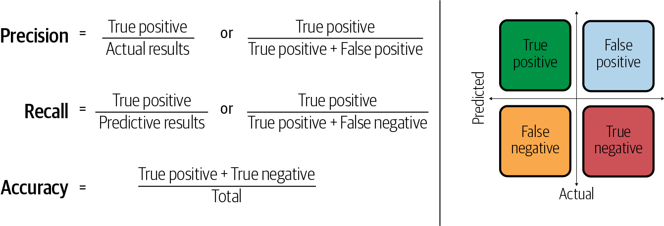
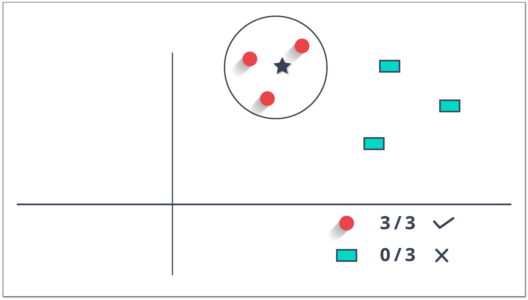
The difference between three commonly used evaluation metrics for classification, accuracy, precision, and recall, is illustrated in Figure 4-8.

Accuracy

As shown in Figure 4-8, accuracy is the number of correct predictions made as a ratio of all predictions made. This is the most common evaluation metric for classification problems and is also the most misused. It is most suitable when there are an equal number of observations in each class (which is rarely the case) and when all predictions and the related prediction errors are equally important, which is often not the case.

Precision

Precision is the percentage of positive instances out of the total predicted positive instances. Here, the denominator is the model prediction done as positive from the whole given dataset. Precision is a good measure to determine when the cost of false positives is high (e.g., email spam detection).

Recall

Recall (or sensitivity or true positive rate) is the percentage of positive instances out of the total actual positive instances. Therefore, the denominator (true positive + false negative) is the actual number of positive instances present in the dataset. Recall is a good measure when there is a high cost associated with false negatives (e.g., fraud detection).

In addition to accuracy, precision, and recall, some of the other commonly used evaluation metrics for classification are discussed in the following sections.

Area under ROC curve

Area under ROC curve (AUC) is an evaluation metric for binary classification problems. ROC is a probability curve, and AUC represents degree or measure of separability. It tells how much the model is capable of distinguishing between classes. The higher the AUC, the better the model is at predicting zeros as zeros and ones as ones. An AUC of 0.5 means that the model has no class separation capacity whatsoever. The probabilistic interpretation of the AUC score is that if you randomly choose a positive case and a negative case, the probability that the positive case outranks the negative case according to the classifier is given by the AUC.

Confusion matrix

A confusion matrix lays out the performance of a learning algorithm. The confusion matrix is simply a square matrix that reports the counts of the true positive (TP), true negative (TN), false positive (FP), and false negative (FN) predictions of a classifier, as shown in Figure 4-9.

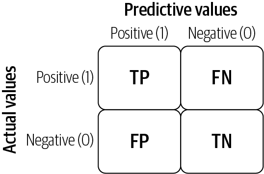
The confusion matrix is a handy presentation of the accuracy of a model with two or more classes. The table presents predictions on the x-axis and accuracy outcomes on the y-axis. The cells of the table are the number of predictions made by the model. For example, a model can predict zero or one, and each prediction may actually have been a zero or a one. Predictions for zero that were actually zero appear in the cell for prediction = 0 and actual = 0, whereas predictions for zero that were actually one appear in the cell for prediction = 0 and actual = 1.

Selecting an evaluation metric for supervised classification

The evaluation metric for classification depends heavily on the task at hand. For example, recall is a good measure when there is a high cost associated with false negatives such as fraud detection. We will further examine these evaluation metrics in the case studies.

Model Selection

Selecting the perfect machine learning model is both an art and a science. Looking at machine learning models, there is no one solution or approach that fits all. There are several factors that can affect your choice of a machine learning model. The main criteria in most of the cases is the model performance that we discussed in the previous section. However, there are many other factors to consider while performing model selection. In the following section, we will go over all such factors, followed by a discussion of model trade-offs.

Factors for Model Selection

The factors considered for the model selection process are as follows:Simplicity

The degree of simplicity of the model. Simplicity usually results in quicker, more scalable, and easier to understand models and results.Training time

Speed, performance, memory usage and overall time taken for model training.Handle nonlinearity in the data

The ability of the model to handle the nonlinear relationship between the variables.Robustness to overfitting

The ability of the model to handle overfitting.Size of the dataset

The ability of the model to handle large number of training examples in the dataset.Number of features

The ability of the model to handle high dimensionality of the feature space.Model interpretation

How explainable is the model? Model interpretability is important because it allows us to take concrete actions to solve the underlying problem.Feature scaling

Does the model require variables to be scaled or normally distributed?

Figure 4-10 compares the supervised learning models on the factors mentioned previously and outlines a general rule-of-thumb to narrow down the search for the best machine learning algorithm⁷ for a given problem. The table is based on the advantages and disadvantages of different models discussed in the individual model section in this chapter.

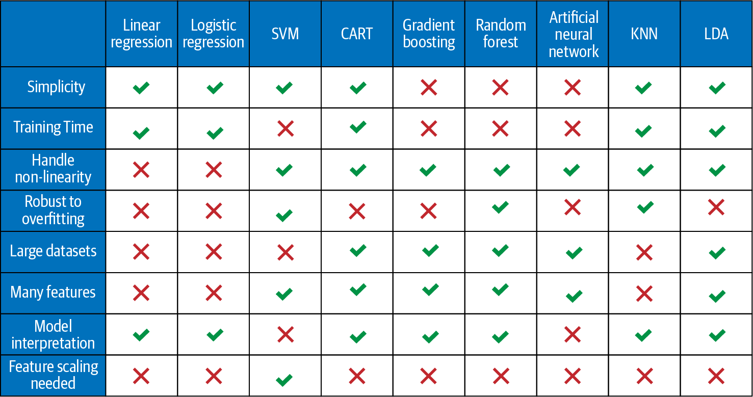
We can see from the table that relatively simple models include linear and logistic regression and as we move towards the ensemble and ANN, the complexity increases. In terms of the training time, the linear models and CART are relatively faster to train as compared to ensemble methods and ANN.

Linear and logistic regression can’t handle nonlinear relationships, while all other models can. SVM can handle the nonlinear relationship between dependent and independent variables with nonlinear kernels.

SVM and random forest tend to overfit less as compared to the linear regression, logistic regression, gradient boosting, and ANN. The degree of overfitting also depends on other parameters, such as size of the data and model tuning, and can be checked by looking at the results of the test set for each model. Also, the boosting methods such as gradient boosting have higher overfitting risk compared to the bagging methods, such as random forest. Recall the focus of gradient boosting is to minimize the bias and not variance.

Linear and logistic regressions are not able to handle large datasets and large number of features well. However, CART, ensemble methods, and ANN are capable of handling large datasets and many features quite well. The linear and logistic regression generally perform better than other models in case the size of the dataset is small. Application of variable reduction techniques (shown in Chapter 7) enables the linear models to handle large datasets. The performance of ANN increases with an increase in the size of the dataset.

Given linear regression, logistic regression, and CART are relatively simpler models, they have better model interpretation as compared to the ensemble models and ANN.

Model Trade-off

Often, it’s a trade-off between different factors when selecting a model. ANN, SVM, and some ensemble methods can be used to create very accurate predictive models, but they may lack simplicity and interpretability and may take a significant amount of resources to train.

In terms of selecting the final model, models with lower interpretability may be preferred when predictive performance is the most important goal, and it’s not necessary to explain how the model works and makes predictions. In some cases, however, model interpretability is mandatory.

Interpretability-driven examples are often seen in the financial industry. In many cases, choosing a machine learning algorithm has less to do with the optimization or the technical aspects of the algorithm and more to do with business decisions. Suppose a machine learning algorithm is used to accept or reject an individual’s credit card application. If the applicant is rejected and decides to file a complaint or take legal action, the financial institution will need to explain how that decision was made. While that can be nearly impossible for ANN, it’s relatively straightforward for decision tree–based models.

Different classes of models are good at modeling different types of underlying patterns in data. So a good first step is to quickly test out a few different classes of models to know which ones capture the underlying structure of the dataset most efficiently. We will follow this approach while performing model selection in all our supervised learning–based case studies.

Chapter Summary

In this chapter, we discussed the importance of supervised learning models in finance, followed by a brief introduction to several supervised learning models, including linear and logistic regression, SVM, decision trees, ensemble, KNN, LDA, and ANN. We demonstrated training and tuning of these models in a few lines of code using sklearn and Keras libraries.

We discussed the most common error metrics for regression and classification models, explained the bias-variance trade-off, and illustrated the various tools for managing the model selection process using cross validation.

We introduced the strengths and weaknesses of each model and discussed the factors to consider when selecting the best model. We also discussed the trade-off between model performance and interpretability.

In the following chapter, we will dive into the case studies for regression and classification. All case studies in the next two chapters leverage the concepts presented in this chapter and in the previous two chapters.

Cross validation will be covered in detail later in this chapter.

See the activation function section of Chapter 3 for details on the sigmoid function.

MLE is a method of estimating the parameters of a probability distribution so that under the assumed statistical model the observed data is most probable.

The approach of projecting data is similar to the PCA algorithm discussed in Chapter 7.

Bias and variance are described in detail later in this chapter.

Split is the process of converting a nonhomogeneous parent node into two homogeneous child nodes best possible).

In this table we do not include AdaBoost and extra trees as their overall behavior across all the parameters are similar to Gradient Boosting and Random Forest, respectively.

Table of Contents

1. What Is a Machine Learning Algorithm?
2. Types of ML Algorithms: Choose Your Fighter
   1. Unsupervised ML Algorithms
      1. Clustering
      2. Dimensionality Reduction
   2. Supervised ML Algorithms
      1. Regression
      2. Classification
      3. Forecasting
   3. Semi-Supervised ML Algorithms
   4. Reinforcement ML Algorithms
3. 5 Simple Steps to Choose the Best Machine Learning Algorithm That Fits Your AI Project Needs
   1. Step 1. Understand Your Project Goal
   2. Step 2. Analyze Your Data by Size, Processing, and Annotation Required
   3. Step 3. Evaluate the Speed and Training Time
   4. Step 4. Find Out the Linearity of Your Data
   5. Step 5. Decide on the Number of Features and Parameters
4. TL;DR

The variety of tasks that machine learning can help you with may be overwhelming. Despite this, the majority of tasks can be solved using a limited number of ML algorithms. Still, you need to know, which of them to choose, when to use them, what parameters to take into consideration, and how to test the ML algorithms. We’ve composed this guide to help you with this specific problem in a pragmatic and easy way.

What Is a Machine Learning Algorithm?

Let’s start with the basics in case you’re still a bit in the dark about what this all is and why you might need it. We’ll talk about what machine learning is and what types of algorithms there are. If you feel like you already know this, you can skip to the step-by-step guide on choosing ML algorithms.

Machine learning is an algorithm-based method for analyzing data with the goal of looking for patterns and making accurate predictions. As the name suggests, ML algorithms are basically computers trained in different ways. These ways are the types of ML algorithms that fall into three and a half broad categories (we’ll explain the “and a half” part a bit later, be patient).

Humanity creates more and more data every day. It comes from a variety of sources: business data, personal social media activity, sensors of IoT, etc. Machine learning algorithms are used to take this data and turn it into something useful that can serve to automate processes, personalize experiences, and make complex predictions that human brains cannot do on their own.

Given the variety of tasks that ML algorithms solve, each type specializes in certain tasks, taking into consideration the features of the data that you have and the requirements of your project. Let’s take a look at each of the major types of ML algorithms and certain examples used for the most common tasks.

Types of ML Algorithms: Choose Your Fighter

There are three major types of ML algorithms: unsupervised, supervised, and reinforcement. An additional one (that we previously counted as “and a half”) is semi-supervised and comes from the combination of supervised and unsupervised. We’ll talk about the unique features and examples of each of these types.

Unsupervised ML Algorithms

This type of machine learning algorithm arguably represents artificial intelligence in its true form. Unsupervised ML is based on the idea that a machine can learn without any guidance from humans. For learning, it uses unlabeled data, which is basically raw data that can be found “in the wild” and is usually unstructured and unprocessed.

Naturally, unsupervised machine learning algorithms have a lot of limitations. As they don’t have any starting point for their training, there are only a few types of tasks that they can perform. The two major ones that we’ll highlight are clustering and dimensionality reduction.

Clustering

While a clustering algorithm won’t be able to tell if you show it the photo of a cat, it can definitely learn to tell a cat from a tree. This means that your computer can tell two different things apart based on their naturally different features and put them into separate groups (clusters). At the same time, it won’t be able to tell you what type of object is in each cluster.

Clustering is great for solving tasks such as spam filtering, fraud detection, primary personalization for marketing, hierarchical clustering for document analysis, etc.

Dimensionality Reduction

Look for dimensionality reduction algorithms in projects that deal with the data that has lots of features and/or variables. The major idea behind this type of algorithm is processing and simplification of the data by decreasing the number of features. The dimensionality reduction model reduces the features that are not essential for the task at hand but leaves the structure and main features of the data intact.

Noise reduction and data visualization are common tasks for dimensionality reduction algorithms. It is also commonly used as an intermediate step in more complex ML projects.

Supervised ML Algorithms

This is arguably the largest and most popular group of machine learning algorithms. And no wonder: supervised learning is flexible, comprehensive, and covers a lot of the common ML tasks that are in high demand today.

In opposition to unsupervised learning, supervised algorithms require labeled data. This means that the models train based on the data that has been processed (cleaned, randomized, and structured) and annotated. The processing and annotation of the data is supervision that a human has over the training process (hence the name of supervised learning).

Annotation, also known as labeling, is an essential process for building a supervised ML algorithm. In a nutshell, it requires adding labels or tags to the pieces of data, which will tell the algorithm how to make sense of it. It’s quite a time-consuming and labor-intensive process that usually gets outsourced to save time for the core business tasks.

There are quite a few interesting algorithm types in supervised learning. For the purposes of brevity, we’ll discuss regression, classification, and forecasting.

Regression

It’s a common case that analysis is required for continuous values to find a correlation between different variables. Regression helps to look for this correlation and predict an output.

This type of supervised algorithm is commonly used to predict the prices or value of certain objects based on a set of their features. Thus, a house will be evaluated based on its location, the number of bedrooms, and if anyone died in it 😉

Classification

Similar to clustering that we’ve already seen in unsupervised machine learning algorithms, classification allows training the AI to group different objects (values) into categories (or classes). The difference is that, now, the machine knows, which class contains which objects. If, after training, you show the computer a photo of a cat and ask what it is, it will tell you it’s a cat and not just group it with other cat photos.

Unlike regression, classification is based on a limited number of values. It can be binary (when there are only two classes, e.g., cats or dogs) or multi-class (when there are more than two categories to classify the values).

Forecasting

When you have past and present data, it’s natural that you’d want to predict the future at some point. Forecasting algorithms can help you with this task as they are able to analyze the data in-depth, looking for hidden patterns, and make predictions based on this analysis.

The trends analysis is obviously the forte of this type of machine learning algorithm. That’s why forecasting is commonly used in business and finance.

Semi-Supervised ML Algorithms

Supervised and unsupervised machine learning algorithms are very common for the majority of AI tasks today. Here’s a simple cheat sheet to facilitate your choice of a machine learning algorithm:

However, sometimes you cannot choose between either an unsupervised or a supervised ML algorithm. There are cases where combining the two algorithms can bring you more benefits even with regard to the growing complexity of your ML model. That’s because of the core features of each type of algorithm: unsupervised learning brings in simplicity and efficiency while supervised learning is all about flexibility and comprehensive goals.

When you combine two different types of algorithms, you get semi-supervised learning. This type of ML algorithm allows you to significantly cut down the financial, human, and time cost for annotating the data. At the same time, semi-supervised learning algorithms are not as restricted in the choice of tasks as supervised learning algorithms.

Reinforcement ML Algorithms

And now for something completely different. Unsupervised and supervised algorithms both work with the data, either unlabeled or labeled. A reinforcement algorithm trains within an environment with a set of rules and a defined goal.

Reinforcement learning algorithms are usually based on dynamic programming techniques. The idea behind this type of ML algorithm is balancing exploration and exploitation. There is some uncharted territory that an algorithm can explore but every action will be followed by a response from a system, either positive or negative. Training on these responses, the algorithm will learn to choose the best set of actions to achieve the set goal.

A classic reinforcement learning application is games such as chess or Go. Learning to play (and win) these games requires the algorithm to understand the environment (the board, the set of rules, and the actions that can be either punished (by the other player taking the pieces) or rewarded (by winning the opponent’s pieces). A more modern and fascinating example of a reinforcement algorithm is training autonomous vehicles. The algorithm is required to navigate the environment without hitting anything and obeying the traffic rules.

5 Simple Steps to Choose the Best Machine Learning Algorithm That Fits Your AI Project Needs

Learning about the different types of machine learning algorithms is not enough to understand how to choose the one that fits your specific purpose. So let’s stick to an incremental method and see how exactly you can approach this problem.

Step 1. Understand Your Project Goal

As it has already become apparent, each machine learning algorithm was designed to solve a specific problem. So, first of all, you should consider the type of project that you’re dealing with.

Answer this question: what kind of an output do you need? Do you need an algorithm for prediction based on the previous data? Turn to supervised forecasting algorithms. Are you looking for an image recognition model that will work with poor-quality photos? Dimensionality reduction in combination with classification will help you with it. Do you need to teach your model to play a new game? A reinforcement algorithm will be your best bet.

Step 2. Analyze Your Data by Size, Processing, and Annotation Required

When you’ve answered the question of what type of output you need, ask yourself what input do you have. What is your data like? Is it raw, just collected from wherever, and requires processing? Is it biased, dirty, and unstructured? Or do you already have a big annotated dataset on your hands? Do you have enough data or is additional collecting (or even collecting from scratch) required? Do you need to spend time preparing your data for the training process or are you good to go?

Insufficient, poor-quality, unprocessed data usually doesn’t lend itself to great training of a supervised algorithm. You should decide if you want to spend time and resources on preparing the best data you can before starting the training process. If not, you can opt for unsupervised algorithms but keep in mind the limitations of such a choice.

Step 3. Evaluate the Speed and Training Time

Here’s another question for you to answer that can help you understand what type of machine learning algorithm you need. Do you need it fast even if it means lower quality of training (and, respectively, predictions)? More and higher-quality data lead to better training. Can you allocate the required time for proper training?

Step 4. Find Out the Linearity of Your Data

Another important question is what the environment of your problem is like? Linear algorithms (such as linear regression or support vector machines) are simpler and faster to train. However, they are not usually used for more complex problems as they deal with linear data. If the data is multifaceted, multidimensional, and has many intersecting correlations, linear algorithms might not be sufficient for your task.

Step 5. Decide on the Number of Features and Parameters

Finally, how complex and accurate your final AI model should be? Don’t forget that longer training usually leads to better, more accurate performance when the AI model is deployed. You can specify more features and parameters for your model to interpret if you have time to let it train longer. So giving your algorithm more time to learn may be a good investment into your future output accuracy and interpretability.

TL;DR

Choosing a machine learning algorithm is obviously a complex task, especially if you don’t have extensive experience in this field. However, learning about the types of algorithms and the tasks that they were designed to solve and answering a set of questions might help you solve this problem. Try to outline as much as you can about:

• Your input (the data: is it collected/sufficient/processed/annotated?)
• Your output (what goal do you pursue?)
• Your field of study (how linear or complex the data is?)
• Your limitations (can you spare time and resources?)
• Your preferences (what features do you absolutely need for success?)

Learning more about machine learning algorithms, their types (from supervised and unsupervised to semi-supervised and reinforcement learning), and answering these questions might lead you to an algorithm that’ll be a perfect match for your goal.

This article will explain some of the most well known machine learning algorithms in less than a minute – helping everyone to understand them!

Linear Regression

One of the simplest Machine learning algorithms out there, Linear Regression is used to make predictions on continuous dependent variables with knowledge from independent variables. A dependent variable is the effect, in which its value depends on changes in the independent variable.

You may remember the line of best fit from school – this is what Linear Regression produces. A simple example is predicting one’s weight depending on their height. 

Logistic Regression

Logistic Regression, similar to Linear Regression, is used to make predictions on categorical dependent variables with knowledge of independent variables. A categorical variable has two or more categories. Logistic Regression classifies outputs that can only be between 0 and 1. 

For example, you can use Logistic Regression to determine whether a student will be admitted or not to a particular college depending on their grades – either Yes or No, or 0 or 1. 

Decision Trees

Decision Trees (DTs) is a probability tree-like structure model that continuously splits data to categorize or make predictions based on the previous set of questions that were answered. The model learns the features of the data and answers questions to help you make better decisions. 

For example, you can use a decision tree using the answers Yes or No to determine a specific species of bird using data features such as feathers, ability to fly or swim, beak type, etc. 

Random Forest

Similar to Decision Trees, Random Forest is also a tree-based algorithm. Where Decision Tree consists of one tree, Random forest uses multiple decision trees for making decisions – a forest of trees. 

It combines multiple models to make predictions and can be used in Classification and Regression tasks. 

K-Nearest Neighbors

K-Nearest Neighbors uses the statistical knowledge of how close a data point is to another data point and determines if these data points can be grouped together. The closeness in the data points reflects the similarities in one another. 

For example, if we had a graph which had a group of data points that were close to one another called Group A and another group of data points that were in close proximity to one another called Group B. When we input a new data point, depending which group the new data point is nearer to – that will be their new classified group. 

Support Vector Machines

Similar to Nearest Neighbor, Support Vector Machines performs classification, regression and outlier detection tasks. It does this by drawing a hyperplane (a straight line) to separate the classes. The data points that are located on one side of the line will be labeled as Group A, whilst the points on the other side will be labeled as Group B.

For example, when a new data point is inputted, depending on which side of the hyperplane and its location within the margin it is – this will determine which group the data point belongs to. 

Naive Bayes

Naive Bayes is based on Bayes’ Theorem which is a mathematical formula used for calculating conditional probabilities. Conditional probability is the chance of an outcome occurring given that another event has also occurred. 

It predicts that the probabilities for each class belongs to a particular class and that the class with the highest probability is considered the most likely class.

k-means Clustering

K-means clustering, similar to nearest neighbors but uses the method of clustering to group similar items/data points in clusters. The number of groups is referred to as K. You do this by selecting the k value, initializing the centroids and then selecting the group and finding the average.

For example, if there are 3 clusters present and a new data point is inputted, depending on which cluster it falls in – that is the cluster they belong to. 

Bagging

Bagging is also known as Bootstrap aggregating and is an ensemble learning technique. Bagging is used in both regression and classification models and aims to avoid overfitting of data and reduce the variance in the predictions. 

Overfitting is when a model fits exactly against its training data – basically not teaching us anything and can be due to various reasons. Random Forest is an example of Bagging. 

Boosting

The overall aim of Boosting is to convert weak learners to strong learners. Weak learners are found by applying base learning algorithms which then generates a new weak prediction rule. A  random sample of data is inputted in a model and then trained sequentially, aiming to train the weak learners and trying to correct its predecessor

XGBoost, which stands for Extreme Gradient Boosting, is used in Boosting.

Dimensionality Reduction

Dimensionality reduction is used to reduce the number of input variables in the training data, by reducing the dimension of your feature set. When a model has a high number of features, it is naturally more complex leading to a higher chance of overfitting and decrease in accuracy. 

For example, if you had a dataset with a hundred columns, dimensionality reduction will reduce the number of columns down to twenty. However, you will need Feature Selection to select relevant features and Feature Engineering to generate new features from existing features.

The Principal Component Analysis (PCA) technique is a type of Dimensionality Reduction. 

Conclusion

The aim of this article was to help you understand Machine Learning algorithms in the most simplest terms. If you would like some more in depth understanding on each of them, have a read of this Popular Machine Learning Algorithms.

We are probably living in the most defining period in technology. The period when computing moved from large mainframes to PCs to self-driving cars and robots. But what makes it defining is not what has happened, but what has gone into getting here. What makes this period exciting is the democratization of the resources and techniques. Data crunching which once took days, today takes mere minutes, all thanks to Machine Learning Algorithms.

This is the reason a Data Scientist gets home a whopping $124,000 a year, increasing the demand forData Science Certifications. 

Let me give you an outline of what this blog will help you understand.

• What is Machine Learning?
• What is a Machine Learning Algorithm?
• What are the types of Machine Learning Algorithms? 
• What is a Supervised Learning Algorithm?
• What is an Unsupervised Learning Algorithm?
• What is a Reinforcement Learning Algorithm?
• List of Machine Learning Algorithms 

Machine Learning Algorithms: What is Machine Learning?

Machine Learning is a concept which allows the machine to learn from examples and experience, and that too without being explicitly programmed.

Let me give you an analogy to make it easier for you to understand.

Let’s suppose one day you went shopping for apples. The vendor had a cart full of apples from where you could handpick the fruit, get it weighed and pay according to the rate fixed (per Kg).

Task: How will you choose the best apples?

Given below is set of learning that a human gains from his experience of shopping for apples, you can drill it down to have a further look at it in detail. Go through it once, you will relate it to machine learning very easily.

Learning 1: Bright red apples are sweeter than pale ones

Learning 2: The smaller and bright red apples are sweet only half the time

Learning 3: Small, pale ones aren’t sweet at all

Learning 4: Crispier apples are juicier

Learning 5: Green apples are tastier than red ones

Learning 6: You don’t need apples anymore

What if you have to write a code for it?

Now, imagine you were asked to write a computer program to choose your apples. You might write the following rules/algorithm:

if (bright red) and if (size is big): Apple is sweet.
if (crispy): Apple is juicy

You would use these rules to choose the apples.

But every time you make a new observation (what if you had to choose oranges, instead) from your experiments, you have to modify the list of rules manually.

You have to understand the details of all the factors affecting the quality of the fruit. If the problem gets complicated enough, it might get difficult for you to make accurate rules by hand that covers all possible types of fruit. This will take a lot of research and effort and not everyone has this amount of time.

This is where Machine Learning Algorithms come into the picture.

So instead of you writing the code, what you do is you feed data to the generic algorithm, and the algorithm/machine builds the logic based on the given data.

Find out our Machine Learning Certification Training Course in Top Cities

India	United States	Other Countries
Machine Learning Training in Dallas	Machine Learning Training in Dallas	Machine Learning Training in Toronto
Machine Learning Course in Hyderabad	Machine Learning Training in Washington	Machine Learning Training in London
Machine Learning Certification in Mumbai	Machine Learning Certification in NYC	Machine Learning Course in Dubai

Machine Learning Algorithms: What is a Machine Learning Algorithm?

Machine Learning algorithm is an evolution of the regular algorithm. It makes your programs “smarter”, by allowing them to automatically learn from the data you provide. The algorithm is mainly divided into:

• Training Phase
• Testing phase

So, building upon the example I had given a while ago, let’s talk a little about these phases.

Training Phase

You take a randomly selected specimen of apples from the market (training data), make a table of all the physical characteristics of each apple, like color, size, shape, grown in which part of the country, sold by which vendor, etc (features), along with the sweetness, juiciness, ripeness of that apple (output variables). You feed this data to the machine learning algorithm (classification/regression), and it learns a model of the correlation between an average apple’s physical characteristics, and its quality.

Testing Phase

Data Science with R Programming Certification Training Course

• Instructor-led Sessions
• Real-life Case Studies
• Assignments
• Lifetime Access

Explore Curriculum

Next time when you go shopping, you will measure the characteristics of the apples which you are purchasing(test data)and feed it to the Machine Learning algorithm. It will use the model which was computed earlier to predict if the apples are sweet, ripe and/or juicy. The algorithm may internally use the rules, similar to the one you manually wrote earlier (for eg, a decision tree). Finally, you can now shop for apples with great confidence, without worrying about the details of how to choose the best apples.

Conclusion 

You know what! you can make your algorithm improve over time (reinforcement learning) so that it will improve its accuracy as it gets trained on more and more training dataset. In case it makes a wrong prediction it will update its rule by itself. 

The best part of this is, you can use the same algorithm to train different models. You can create one each for predicting the quality of mangoes, grapes, bananas, or whichever fruit you want.

For a more detailed explanation on Machine Learning Algorithms feel free to go through this video:

Machine Learning Full Course | Machine Learning Tutorial | Edureka

This Machine Learning Algorithms Tutorial shall teach you what machine learning is, and the various ways in which you can use machine learning to solve a problem!

Let’s categorize Machine Learning Algorithm into subparts and see what each of them are, how they work, and how each one of them is used in real life.

Machine Learning Algorithms: What are the types of Machine Learning Algorithms?

So, Machine Learning Algorithms can be categorized by the following three types.

Machine Learning Algorithms: What is Supervised Learning?

This category is termed as supervised learning because the process of an algorithm learning from the training dataset can be thought of as a teacher teaching his students. The algorithm continuously predicts the result on the basis of training data and is continuously corrected by the teacher. The learning continues until the algorithm achieves an acceptable level of performance.

Let me rephrase you this in simple terms:

In Supervised machine learning algorithm, every instance of the training dataset consists of input attributes and expected output. The training dataset can take any kind of data as input like values of a database row, the pixels of an image, or even an audio frequency histogram. 

Example: In Biometric Attendance you can train the machine with inputs of your biometric identity – it can be your thumb, iris or ear-lobe, etc. Once the machine is trained it can validate your future input and can easily identify you.

Machine Learning Algorithms: What is Unsupervised Learning? 

Well, this category of machine learning is known as unsupervised because unlike supervised learning there is no teacher. Algorithms are left on their own to discover and return the interesting structure in the data.

The goal for unsupervised learning is to model the underlying structure or distribution in the data in order to learn more about the data.

Let me rephrase it for you in simple terms:

In the unsupervised learning approach, the sample of a training dataset does not have an expected output associated with them. Using the unsupervised learning algorithms you can detect patterns based on the typical characteristics of the input data. Clustering can be considered as an example of a machine learning task that uses the unsupervised learning approach. The machine then groups similar data samples and identify different clusters within the data.

Example: Fraud Detection is probably the most popular use-case of Unsupervised Learning. Utilizing past historical data on fraudulent claims, it is possible to isolate new claims based on its proximity to clusters that indicate fraudulent patterns. 

Also, enroll in Artificial Intelligence and Machine Learning courses to become proficient in this AI and ML.

Machine Learning Algorithms: What is Reinforcement Learning?

Reinforcement learning can be thought of like a hit and trial method of learning. The machine gets a Reward or Penalty point for each action it performs. If the option is correct, the machine gains the reward point or gets a penalty point in case of a wrong response.

The reinforcement learning algorithm is all about the interaction between the environment and the learning agent. The learning agent is based on exploration and exploitation.

Exploration is when the learning agent acts on trial and error and Exploitation is when it performs an action based on the knowledge gained from the environment. The environment rewards the agent for every correct action, which is the reinforcement signal. With the aim of collecting more rewards obtained, the agent improves its environment knowledge to choose or perform the next action.

Let see how Pavlov trained his dog using reinforcement training?

Pavlov divided the training of his dog into three stages.

Stage 1: In the first part, Pavlov gave meat to the dog, and in response to the meat, the dog started salivating.

Stage 2: In the next stage he created a sound with a bell, but this time the dogs did not respond to anything.

Stage 3: In the third stage, he tried to train his dog by using the bell and then giving them food. Seeing the food the dog started salivating.

Eventually, the dogs started salivating just after hearing the bell, even if the food was not given as the dog was reinforced that whenever the master will ring the bell, he will get the food. Reinforcement Learning is a continuous process, either by stimulus or feedback.

Machine Learning Algorithms: List of Machine Learning Algorithms 

Here is the list of 5 most commonly used machine learning algorithms. 

1. Linear Regression
2. Logistic Regression
3. Decision Tree
4. Naive Bayes
5. kNN

1. Linear Regression

It is used to estimate real values (cost of houses, number of calls, total sales etc.) based on continuous variables. Here, we establish a relationship between the independent and dependent variables by fitting the best line. This best fit line is known as the regression line and represented by a linear equation Y= aX + b.

The best way to understand linear regression is to relive this experience of childhood. Let us say, you ask a child in fifth grade to arrange people in his class by increasing order of weight, without asking them their weights! What do you think the child will do? He/she would likely look (visually analyze) at the height and build of people and arrange them using a combination of these visible parameters. This is a linear regression in real life! The child has actually figured out that height and build would be correlated to the weight by a relationship, which looks like the equation above.

In this equation:

• Y – Dependent Variable
• a – Slope
• X – Independent variable
• b – Intercept

These coefficients a and b are derived based on minimizing the ‘sum of squared differences’ of distance between data points and regression line.

Look at the plot given. Here, we have identified the best fit having linear equation y=0.2811x+13.9. Now using this equation, we can find the weight, knowing the height of a person.

R-Code:

#Load Train and Test datasets
#Identify feature and response variable(s) and values must be numeric and numpy arrays
x_train <- input_variables_values_training_datasets
y_train <- target_variables_values_training_datasets
x_test <- input_variables_values_test_datasets
x <- cbind(x_train,y_train)
# Train the model using the training sets and check score
linear <- lm(y_train ~ ., data = x)
summary(linear)
#Predict Output
predicted= predict(linear,x_test) 

2. Logistic Regression

Don’t get confused by its name! It is a classification, and not a regression algorithm. It is used to estimate discrete values ( Binary values like 0/1, yes/no, true/false ) based on a given set of independent variable(s). In simple words, it predicts the probability of occurrence of an event by fitting data to a logit function. Hence, it is also known as logit regression. Since it predicts the probability, its output values lie between 0 and 1.

Again, let us try and understand this through a simple example.

Let’s say your friend gives you a puzzle to solve. There are only 2 outcome scenarios – either you solve it or you don’t. Now imagine, that you are being given a wide range of puzzles/quizzes in an attempt to understand which subjects you are good at. The outcome of this study would be something like this – if you are given a trigonometry based tenth-grade problem, you are 70% likely to solve it. On the other hand, if it is grade fifth history question, the probability of getting an answer is only 30%. This is what Logistic Regression provides you.

Coming to the math, the log odds of the outcome is modeled as a linear combination of the predictor variables.

odds= p/ (1-p) = probability of event occurrence / probability of not event occurrence ln(odds) = ln(p/(1-p)) logit(p) = ln(p/(1-p)) = b0+b1X1+b2X2+b3X3....+bkXk

Above, p is the probability of the presence of the characteristic of interest. It chooses parameters that maximize the likelihood of observing the sample values rather than that minimize the sum of squared errors (like in ordinary regression).

Now, you may ask, why take a log? For the sake of simplicity, let’s just say that this is one of the best mathematical ways to replicate a step function. I can go in more details, but that will beat the purpose of this blog.

R-Code:

x <- cbind(x_train,y_train)
# Train the model using the training sets and check score
logistic <- glm(y_train ~ ., data = x,family='binomial')
summary(logistic)
#Predict Output
predicted= predict(logistic,x_test)

There are many different steps that could be tried in order to improve the model:

• including interaction terms
• removing features
• regularization techniques
• using a non-linear model

3. Decision Tree

Now, this is one of my favorite algorithms. It is a type of supervised learning algorithm that is mostly used for classification problems. Surprisingly, it works for both categorical and continuous dependent variables. In this algorithm, we split the population into two or more homogeneous sets. This is done based on the most significant attributes/ independent variables to make as distinct groups as possible.

In the image above, you can see that population is classified into four different groups based on multiple attributes to identify ‘if they will play or not’. 

R-Code:

library(rpart)
x <- cbind(x_train,y_train)
# grow tree 
fit <- rpart(y_train ~ ., data = x,method="class")
summary(fit)
#Predict Output 
predicted= predict(fit,x_test)

4. Naive Bayes

This is a classification technique based on Bayes’ theorem with an assumption of independence between predictors. In simple terms, a Naive Bayes classifier assumes that the presence of a particular feature in a class is unrelated to the presence of any other feature.

For example, a fruit may be considered to be an apple if it is red, round, and about 3 inches in diameter. Even if these features depend on each other or upon the existence of the other features, a naive Bayes classifier would consider all of these properties to independently contribute to the probability that this fruit is an apple.

Naive Bayesian model is easy to build and particularly useful for very large data sets. Along with simplicity, Naive Bayes is known to outperform even highly sophisticated classification methods.

Bayes theorem provides a way of calculating posterior probability P(c|x) from P(c), P(x) and P(x|c). Look at the equation below:

Here,

• P(c|x) is the posterior probability of class (target) given predictor (attribute). 
• P(c) is the prior probability of class. 
• P(x|c) is the likelihood which is the probability of predictor given class. 
• P(x) is the prior probability of predictor.

Example: Let’s understand it using an example. Below I have a training data set of weather and corresponding target variable ‘Play’. Now, we need to classify whether players will play or not based on weather condition. Let’s follow the below steps to perform it.

Step 1: Convert the data set to the frequency table

Step 2: Create a Likelihood table by finding the probabilities like Overcast probability = 0.29 and probability of playing is 0.64.

Step 3: Now, use the Naive Bayesian equation to calculate the posterior probability for each class. The class with the highest posterior probability is the outcome of prediction.

Problem: Players will pay if the weather is sunny, is this statement is correct?

We can solve it using above discussed method, so P(Yes | Sunny) = P( Sunny | Yes) * P(Yes) / P (Sunny)

Here we have P (Sunny |Yes) = 3/9 = 0.33, P(Sunny) = 5/14 = 0.36, P( Yes)= 9/14 = 0.64

Now, P (Yes | Sunny) = 0.33 * 0.64 / 0.36 = 0.60, which has higher probability.

Data Science with R Programming Certification Training Course

Weekday / Weekend BatchesSee Batch Details

Naive Bayes uses a similar method to predict the probability of different class based on various attributes. This algorithm is mostly used in text classification and with problems having multiple classes.

R-Code:

library(e1071)
x <- cbind(x_train,y_train)
# Fitting model
fit <-naiveBayes(y_train ~ ., data = x)
summary(fit)
#Predict Output 
predicted= predict(fit,x_test)

5. kNN (k- Nearest Neighbors)

It can be used for both classification and regression problems. However, it is more widely used in classification problems in the industry. K nearest neighbors is a simple algorithm that stores all available cases and classifies new cases by a majority vote of its k neighbors. The case being assigned to the class is most common amongst its K nearest neighbors measured by a distance function.

These distance functions can be Euclidean, Manhattan, Minkowski and Hamming distance. First three functions are used for continuous function and the fourth one (Hamming) for categorical variables. If K = 1, then the case is simply assigned to the class of its nearest neighbor. At times, choosing K turns out to be a challenge while performing kNN modeling.

KNN can easily be mapped to our real lives. If you want to learn about a person, of whom you have no information, you might like to find out about his close friends and the circles he moves in and gain access to his/her information!

R-Code:

library(knn)
x <- cbind(x_train,y_train)
# Fitting model
fit <-knn(y_train ~ ., data = x,k=5)
summary(fit)
#Predict Output 
predicted= predict(fit,x_test)

Things to consider before selecting KNN:

• KNN is computationally expensive
• Variables should be normalized else higher range variables can bias it
• Works on pre-processing stage more before going for kNN like an outlier, noise removal

This brings me to the end of this blog. Stay tuned for more content on Machine Learning and Data Science!

Are you wondering how to advance once you know the basics of what Machine Learning is? Take a look at Edureka’s Machine Learning Certification, which will help you get on the right path to succeed in this fascinating field. Learn the fundamentals of Machine Learning, machine learning steps and methods that include unsupervised and supervised learning, mathematical and heuristic aspects, and hands-on modeling to create algorithms. You will be prepared for the position of Machine Learning engineer.

You can also take a Machine Learning Course Masters Program. The program will provide you with the most in-depth and practical information on machine-learning applications in real-world situations. Additionally, you’ll learn the essentials needed to be successful in the field of machine learning, such as statistical analysis, Python, and data science.

Machine learning (ML) is rapidly changing the world, from diverse types of applications and research pursued in industry and academia. Machine learning is affecting every part of our daily lives. From voice assistants using NLP and machine learning to make appointments, check our calendar, and play music, to programmatic advertisements — that are so accurate that they can predict what we will need before we even think of it.

More often than not, the complexity of the scientific field of machine learning can be overwhelming, making keeping up with “what is important” a very challenging task. However, to make sure that we provide a learning path to those who seek to learn machine learning, but are new to these concepts. In this article, we look at the most critical basic algorithms that hopefully make your machine learning journey less challenging.

Any suggestions or feedback is crucial to continue to improve. Please let us know in the comments if you have any.

Index

• Introduction to Machine Learning.
• Major Machine Learning Algorithms.
• Supervised vs. Unsupervised Learning.
• Linear Regression.
• Multivariable Linear Regression.
• Polynomial Regression.
• Exponential Regression.
• Sinusoidal Regression.
• Logarithmic Regression.

What is machine learning?

A computer program is said to learn from experience E with respect to some class of tasks T and performance measure P, if its performance at tasks in T, as measured by P, improves with experience E. ~ Tom M. Mitchell [1]

Machine learning behaves similarly to the growth of a child. As a child grows, her experience E in performing task T increases, which results in higher performance measure (P).

For instance, we give a “shape sorting block” toy to a child. (Now we all know that in this toy, we have different shapes and shape holes). In this case, our task T is to find an appropriate shape hole for a shape. Afterward, the child observes the shape and tries to fit it in a shaped hole. Let us say that this toy has three shapes: a circle, a triangle, and a square. In her first attempt at finding a shaped hole, her performance measure(P) is 1/3, which means that the child found 1 out of 3 correct shape holes.

Second, the child tries it another time and notices that she is a little experienced in this task. Considering the experience gained (E), the child tries this task another time, and when measuring the performance(P), it turns out to be 2/3. After repeating this task (T) 100 times, the baby now figured out which shape goes into which shape hole.

So her experience (E) increased, her performance(P) also increased, and then we notice that as the number of attempts at this toy increases. The performance also increases, which results in higher accuracy.

Such execution is similar to machine learning. What a machine does is, it takes a task (T), executes it, and measures its performance (P). Now a machine has a large number of data, so as it processes that data, its experience (E) increases over time, resulting in a higher performance measure (P). So after going through all the data, our machine learning model’s accuracy increases, which means that the predictions made by our model will be very accurate.

Another definition of machine learning by Arthur Samuel:

Machine Learning is the subfield of computer science that gives “computers the ability to learn without being explicitly programmed.” ~ Arthur Samuel [2]

Let us try to understand this definition: It states “learn without being explicitly programmed” — which means that we are not going to teach the computer with a specific set of rules, but instead, what we are going to do is feed the computer with enough data and give it time to learn from it, by making its own mistakes and improve upon those. For example, We did not teach the child how to fit in the shapes, but by performing the same task several times, the child learned to fit the shapes in the toy by herself.

Therefore, we can say that we did not explicitly teach the child how to fit the shapes. We do the same thing with machines. We give it enough data to work on and feed it with the information we want from it. So it processes the data and predicts the data accurately.

Why do we need machine learning?

For instance, we have a set of images of cats and dogs. What we want to do is classify them into a group of cats and dogs. To do that we need to find out different animal features, such as:

1. How many eyes does each animal have?
2. What is the eye color of each animal?
3. What is the height of each animal?
4. What is the weight of each animal?
5. What does each animal generally eat?

We form a vector on each of these questions’ answers. Next, we apply a set of rules such as:

If height > 1 feet and weight > 15 lbs, then it could be a cat.

Now, we have to make such a set of rules for every data point. Furthermore, we place a decision tree of if, else if, else statements and check whether it falls into one of the categories.

Let us assume that the result of this experiment was not fruitful as it misclassified many of the animals, which gives us an excellent opportunity to use machine learning.

What machine learning does is process the data with different kinds of algorithms and tells us which feature is more important to determine whether it is a cat or a dog. So instead of applying many sets of rules, we can simplify it based on two or three features, and as a result, it gives us a higher accuracy. The previous method was not generalized enough to make predictions.

Machine learning models helps us in many tasks, such as:

• Object Recognition
• Summarization
• Prediction
• Classification
• Clustering
• Recommender systems
• And others

What is a machine learning model?

A machine learning model is a question/answering system that takes care of processing machine-learning related tasks. Think of it as an algorithm system that represents data when solving problems. The methods we will tackle below are beneficial for industry-related purposes to tackle business problems.

For instance, let us imagine that we are working on Google Adwords’ ML system, and our task is to implementing an ML algorithm to convey a particular demographic or area using data. Such a task aims to go from using data to gather valuable insights to improve business outcomes.

Major Machine Learning Algorithms:

1. Regression (Prediction)

We use regression algorithms for predicting continuous values.

Regression algorithms:

• Linear Regression
• Polynomial Regression
• Exponential Regression
• Logistic Regression
• Logarithmic Regression

2. Classification

We use classification algorithms for predicting a set of items’ class or category.

Classification algorithms:

• K-Nearest Neighbors
• Decision Trees
• Random Forest
• Support Vector Machine
• Naive Bayes

3. Clustering

We use clustering algorithms for summarization or to structure data.

Clustering algorithms:

• K-means
• DBSCAN
• Mean Shift
• Hierarchical

4. Association

We use association algorithms for associating co-occurring items or events.

Association algorithms:

• Apriori

5. Anomaly Detection

We use anomaly detection for discovering abnormal activities and unusual cases like fraud detection.

6. Sequence Pattern Mining

We use sequential pattern mining for predicting the next data events between data examples in a sequence.

7. Dimensionality Reduction

We use dimensionality reduction for reducing the size of data to extract only useful features from a dataset.

8. Recommendation Systems

We use recommenders algorithms to build recommendation engines.

Examples:

• Netflix recommendation system.
• A book recommendation system.
• A product recommendation system on Amazon.

Nowadays, we hear many buzz words like artificial intelligence, machine learning, deep learning, and others.

What are the fundamental differences between Artificial Intelligence, Machine Learning, and Deep Learning?

Artificial Intelligence (AI):

Artificial intelligence (AI), as defined by Professor Andrew Moore, is the science and engineering of making computers behave in ways that, until recently, we thought required human intelligence [4].

These include:

• Computer Vision
• Language Processing
• Creativity
• Summarization

Machine Learning (ML):

As defined by Professor Tom Mitchell, machine learning refers to a scientific branch of AI, which focuses on the study of computer algorithms that allow computer programs to automatically improve through experience [3].

These include:

• Classification
• Neural Network
• Clustering

Deep Learning:

Deep learning is a subset of machine learning in which layered neural networks, combined with high computing power and large datasets, can create powerful machine learning models. [3]

Why do we prefer Python to implement machine learning algorithms?

Python is a popular and general-purpose programming language. We can write machine learning algorithms using Python, and it works well. The reason why Python is so popular among data scientists is that Python has a diverse variety of modules and libraries already implemented that make our life more comfortable.

Let us have a brief look at some exciting Python libraries.

1. Numpy: It is a math library to work with n-dimensional arrays in Python. It enables us to do computations effectively and efficiently.
2. Scipy: It is a collection of numerical algorithms and domain-specific tool-box, including signal processing, optimization, statistics, and much more. Scipy is a functional library for scientific and high-performance computations.
3. Matplotlib: It is a trendy plotting package that provides 2D plotting as well as 3D plotting.
4. Scikit-learn: It is a free machine learning library for python programming language. It has most of the classification, regression, and clustering algorithms, and works with Python numerical libraries such as Numpy, Scipy.

Machine learning algorithms classify into two groups :

• Supervised Learning algorithms
• Unsupervised Learning algorithms

I. Supervised Learning Algorithms:

Goal: Predict class or value label.

Supervised learning is a branch of machine learning(perhaps it is the mainstream of machine/deep learning for now) related to inferring a function from labeled training data. Training data consists of a set of *(input, target)* pairs, where the input could be a vector of features, and the target instructs what we desire for the function to output. Depending on the type of the *target*, we can roughly divide supervised learning into two categories: classification and regression. Classification involves categorical targets; examples ranging from some simple cases, such as image classification, to some advanced topics, such as machine translations and image caption. Regression involves continuous targets. Its applications include stock prediction, image masking, and others- which all fall in this category.

To understand what supervised learning is, we will use an example. For instance, we give a child 100 stuffed animals in which there are ten animals of each kind like ten lions, ten monkeys, ten elephants, and others. Next, we teach the kid to recognize the different types of animals based on different characteristics (features) of an animal. Such as if its color is orange, then it might be a lion. If it is a big animal with a trunk, then it may be an elephant.

We teach the kid how to differentiate animals, this can be an example of supervised learning. Now when we give the kid different animals, he should be able to classify them into an appropriate animal group.

For the sake of this example, we notice that 8/10 of his classifications were correct. So we can say that the kid has done a pretty good job. The same applies to computers. We provide them with thousands of data points with its actual labeled values (Labeled data is classified data into different groups along with its feature values). Then it learns from its different characteristics in its training period. After the training period is over, we can use our trained model to make predictions. Keep in mind that we already fed the machine with labeled data, so its prediction algorithm is based on supervised learning. In short, we can say that the predictions by this example are based on labeled data.

Example of supervised learning algorithms :

• Linear Regression
• Logistic Regression
• K-Nearest Neighbors
• Decision Tree
• Random Forest
• Support Vector Machine

II. Unsupervised Learning:

Goal: Determine data patterns/groupings.

In contrast to supervised learning. Unsupervised learning infers from unlabeled data, a function that describes hidden structures in data.

Perhaps the most basic type of unsupervised learning is dimension reduction methods, such as PCA, t-SNE, while PCA is generally used in data preprocessing, and t-SNE usually used in data visualization.

A more advanced branch is clustering, which explores the hidden patterns in data and then makes predictions on them; examples include K-mean clustering, Gaussian mixture models, hidden Markov models, and others.

Along with the renaissance of deep learning, unsupervised learning gains more and more attention because it frees us from manually labeling data. In light of deep learning, we consider two kinds of unsupervised learning: representation learning and generative models.

Representation learning aims to distill a high-level representative feature that is useful for some downstream tasks, while generative models intend to reproduce the input data from some hidden parameters.

Unsupervised learning works as it sounds. In this type of algorithms, we do not have labeled data. So the machine has to process the input data and try to make conclusions about the output. For example, remember the kid whom we gave a shape toy? In this case, he would learn from its own mistakes to find the perfect shape hole for different shapes.

But the catch is that we are not feeding the child by teaching the methods to fit the shapes (for machine learning purposes called labeled data). However, the child learns from the toy’s different characteristics and tries to make conclusions about them. In short, the predictions are based on unlabeled data.

Examples of unsupervised learning algorithms:

• Dimension Reduction
• Density Estimation
• Market Basket Analysis
• Generative adversarial networks (GANs)
• Clustering

For this article, we will use a few types of regression algorithms with coding samples in Python.

1. Linear Regression:

Linear regression is a statistical approach that models the relationship between input features and output. The input features are called the independent variables, and the output is called a dependent variable. Our goal here is to predict the value of the output based on the input features by multiplying it with its optimal coefficients.

Some real-life examples of linear regression :

(1) To predict sales of products.

(2) To predict economic growth.

(3) To predict petroleum prices.

(4) To predict the emission of a new car.

(5) Impact of GPA on college admissions.

There are two types of linear regression :

1. Simple Linear Regression
2. Multivariable Linear Regression

1.1 Simple Linear Regression:

In simple linear regression, we predict the output/dependent variable based on only one input feature. The simple linear regression is given by:

Below we are going to implement simple linear regression using the sklearn library in Python.

Step by step implementation in Python:

a. Import required libraries:

Since we are going to use various libraries for calculations, we need to import them.

b. Read the CSV file:

We check the first five rows of our dataset. In this case, we are using a vehicle model dataset — please check out the dataset on Softlayer IBM.

c. Select the features we want to consider in predicting values:

Here our goal is to predict the value of “co2 emissions” from the value of “engine size” in our dataset.

d. Plot the data:

We can visualize our data on a scatter plot.

e. Divide the data into training and testing data:

To check the accuracy of a model, we are going to divide our data into training and testing datasets. We will use training data to train our model, and then we will check the accuracy of our model using the testing dataset.

f. Training our model:

Here is how we can train our model and find the coefficients for our best-fit regression line.

g. Plot the best fit line:

Based on the coefficients, we can plot the best fit line for our dataset.

h. Prediction function:

We are going to use a prediction function for our testing dataset.

i. Predicting co2 emissions:

Predicting the values of co2 emissions based on the regression line.

j. Checking accuracy for test data :

We can check the accuracy of a model by comparing the actual values with the predicted values in our dataset.

Putting it all together:

# Import required libraries:
import pandas as pd
import numpy as np
import matplotlib.pyplot as plt
from sklearn import linear_model# Read the CSV file :
data = pd.read_csv(“Fuel.csv”)
data.head()# Let’s select some features to explore more :
data = data[[“ENGINESIZE”,”CO2EMISSIONS”]]# ENGINESIZE vs CO2EMISSIONS:
plt.scatter(data[“ENGINESIZE”] , data[“CO2EMISSIONS”] , color=”blue”)
plt.xlabel(“ENGINESIZE”)
plt.ylabel(“CO2EMISSIONS”)
plt.show()# Generating training and testing data from our data:
# We are using 80% data for training.
train = data[:(int((len(data)*0.8)))]
test = data[(int((len(data)*0.8))):]# Modeling:
# Using sklearn package to model data :
regr = linear_model.LinearRegression()
train_x = np.array(train[[“ENGINESIZE”]])
train_y = np.array(train[[“CO2EMISSIONS”]])
regr.fit(train_x,train_y)# The coefficients:
print (“coefficients : “,regr.coef_) #Slope
print (“Intercept : “,regr.intercept_) #Intercept# Plotting the regression line:
plt.scatter(train[“ENGINESIZE”], train[“CO2EMISSIONS”], color=’blue’)
plt.plot(train_x, regr.coef_*train_x + regr.intercept_, ‘-r’)
plt.xlabel(“Engine size”)
plt.ylabel(“Emission”)# Predicting values:
# Function for predicting future values :
def get_regression_predictions(input_features,intercept,slope):
 predicted_values = input_features*slope + intercept
 return predicted_values# Predicting emission for future car:
my_engine_size = 3.5
estimatd_emission = get_regression_predictions(my_engine_size,regr.intercept_[0],regr.coef_[0][0])
print (“Estimated Emission :”,estimatd_emission)# Checking various accuracy:
from sklearn.metrics import r2_score
test_x = np.array(test[[‘ENGINESIZE’]])
test_y = np.array(test[[‘CO2EMISSIONS’]])
test_y_ = regr.predict(test_x)print(“Mean absolute error: %.2f” % np.mean(np.absolute(test_y_ — test_y)))
print(“Mean sum of squares (MSE): %.2f” % np.mean((test_y_ — test_y) ** 2))
print(“R2-score: %.2f” % r2_score(test_y_ , test_y) )

1.2 Multivariable Linear Regression:

In simple linear regression, we were only able to consider one input feature for predicting the value of the output feature. However, in Multivariable Linear Regression, we can predict the output based on more than one input feature. Here is the formula for multivariable linear regression.

Step by step implementation in Python:

a. Import the required libraries:

b. Read the CSV file :

c. Define X and Y:

X stores the input features we want to consider, and Y stores the value of output.

d. Divide data into a testing and training dataset:

Here we are going to use 80% data in training and 20% data in testing.

e. Train our model :

Here we are going to train our model with 80% of the data.

f. Find the coefficients of input features :

Now we need to know which feature has a more significant effect on the output variable. For that, we are going to print the coefficient values. Note that the negative coefficient means it has an inverse effect on the output. i.e., if the value of that features increases, then the output value decreases.

g. Predict the values:

h. Accuracy of the model:

Now notice that here we used the same dataset for simple and multivariable linear regression. We can notice that the accuracy of multivariable linear regression is far better than the accuracy of simple linear regression.

Putting it all together:

# Import the required libraries:
import pandas as pd
import numpy as np
import matplotlib.pyplot as plt
from sklearn import linear_model# Read the CSV file:
data = pd.read_csv(“Fuel.csv”)
data.head()# Consider features we want to work on:
X = data[[ ‘ENGINESIZE’, ‘CYLINDERS’, ‘FUELCONSUMPTION_CITY’,’FUELCONSUMPTION_HWY’, 
 ‘FUELCONSUMPTION_COMB’,’FUELCONSUMPTION_COMB_MPG’]]Y = data[“CO2EMISSIONS”]# Generating training and testing data from our data:
# We are using 80% data for training.
train = data[:(int((len(data)*0.8)))]
test = data[(int((len(data)*0.8))):]#Modeling:
#Using sklearn package to model data :
regr = linear_model.LinearRegression()train_x = np.array(train[[ ‘ENGINESIZE’, ‘CYLINDERS’, ‘FUELCONSUMPTION_CITY’,
 ‘FUELCONSUMPTION_HWY’, ‘FUELCONSUMPTION_COMB’,’FUELCONSUMPTION_COMB_MPG’]])
train_y = np.array(train[“CO2EMISSIONS”])regr.fit(train_x,train_y)test_x = np.array(test[[ ‘ENGINESIZE’, ‘CYLINDERS’, ‘FUELCONSUMPTION_CITY’,
 ‘FUELCONSUMPTION_HWY’, ‘FUELCONSUMPTION_COMB’,’FUELCONSUMPTION_COMB_MPG’]])
test_y = np.array(test[“CO2EMISSIONS”])# print the coefficient values:
coeff_data = pd.DataFrame(regr.coef_ , X.columns , columns=[“Coefficients”])
coeff_data#Now let’s do prediction of data:
Y_pred = regr.predict(test_x)# Check accuracy:
from sklearn.metrics import r2_score
R = r2_score(test_y , Y_pred)
print (“R² :”,R)

1.3 Polynomial Regression:

Sometimes we have data that does not merely follow a linear trend. We sometimes have data that follows a polynomial trend. Therefore, we are going to use polynomial regression.

Before digging into its implementation, we need to know how the graphs of some primary polynomial data look.

Polynomial Functions and Their Graphs:

a. Graph for Y=X:

b. Graph for Y = X²:

c. Graph for Y = X³:

d. Graph with more than one polynomials: Y = X³+X²+X:

In the graph above, we can see that the red dots show the graph for Y=X³+X²+X and the blue dots shows the graph for Y = X³. Here we can see that the most prominent power influences the shape of our graph.

Below is the formula for polynomial regression:

Now in the previous regression models, we used sci-kit learn library for implementation. Now in this, we are going to use Normal Equation to implement it. Here notice that we can use scikit-learn for implementing polynomial regression also, but another method will give us an insight into how it works.

The equation goes as follows:

In the equation above:

θ: hypothesis parameters that define it the best.

X: input feature value of each instance.

Y: Output value of each instance.

1.3.1 Hypothesis Function for Polynomial Regression

The main matrix in the standard equation:

Step by step implementation in Python:

a. Import the required libraries:

b. Generate the data points:

We are going to generate a dataset for implementing our polynomial regression.

c. Initialize x,x²,x³ vectors:

We are taking the maximum power of x as 3. So our X matrix will have X, X², X³.

d. Column-1 of X matrix:

The 1st column of the main matrix X will always be 1 because it holds the coefficient of beta_0.

e. Form the complete x matrix:

Look at the matrix X at the start of this implementation. We are going to create it by appending vectors.

f. Transpose of the matrix:

We are going to calculate the value of theta step-by-step. First, we need to find the transpose of the matrix.

g. Matrix multiplication:

After finding the transpose, we need to multiply it with the original matrix. Keep in mind that we are going to implement it with a normal equation, so we have to follow its rules.

h. The inverse of a matrix:

Finding the inverse of the matrix and storing it in temp1.

i. Matrix multiplication:

Finding the multiplication of transposed X and the Y vector and storing it in the temp2 variable.

j. Coefficient values:

To find the coefficient values, we need to multiply temp1 and temp2. See the Normal Equation formula.

k. Store the coefficients in variables:

Storing those coefficient values in different variables.

l. Plot the data with curve:

Plotting the data with the regression curve.

m. Prediction function:

Now we are going to predict the output using the regression curve.

n. Error function:

Calculate the error using mean squared error function.

o. Calculate the error:

Putting it all together:

# Import required libraries:
import numpy as np
import matplotlib.pyplot as plt# Generate datapoints:
x = np.arange(-5,5,0.1)
y_noise = 20 * np.random.normal(size = len(x))
y = 1*(x**3) + 1*(x**2) + 1*x + 3+y_noise
plt.scatter(x,y)# Make polynomial data:
x1 = x
x2 = np.power(x1,2)
x3 = np.power(x1,3)# Reshaping data:
x1_new = np.reshape(x1,(n,1))
x2_new = np.reshape(x2,(n,1))
x3_new = np.reshape(x3,(n,1))# First column of matrix X:
x_bias = np.ones((n,1))# Form the complete x matrix:
x_new = np.append(x_bias,x1_new,axis=1)
x_new = np.append(x_new,x2_new,axis=1)
x_new = np.append(x_new,x3_new,axis=1)# Finding transpose:
x_new_transpose = np.transpose(x_new)# Finding dot product of original and transposed matrix :
x_new_transpose_dot_x_new = x_new_transpose.dot(x_new)# Finding Inverse:
temp_1 = np.linalg.inv(x_new_transpose_dot_x_new)# Finding the dot product of transposed x and y :
temp_2 = x_new_transpose.dot(y)# Finding coefficients:
theta = temp_1.dot(temp_2)
theta# Store coefficient values in different variables:
beta_0 = theta[0]
beta_1 = theta[1]
beta_2 = theta[2]
beta_3 = theta[3]# Plot the polynomial curve:
plt.scatter(x,y)
plt.plot(x,beta_0 + beta_1*x1 + beta_2*x2 + beta_3*x3,c=”red”)# Prediction function:
def prediction(x1,x2,x3,beta_0,beta_1,beta_2,beta_3):
 y_pred = beta_0 + beta_1*x1 + beta_2*x2 + beta_3*x3
 return y_pred
 
# Making predictions:
pred = prediction(x1,x2,x3,beta_0,beta_1,beta_2,beta_3)
 
# Calculate accuracy of model:
def err(y_pred,y):
 var = (y — y_pred)
 var = var*var
 n = len(var)
 MSE = var.sum()
 MSE = MSE/n
 
 return MSE# Calculating the error:
error = err(pred,y)
error

1.4 Exponential Regression:

Some real-life examples of exponential growth:

1. Microorganisms in cultures.

2. Spoilage of food.

3. Human Population.

4. Compound Interest.

5. Pandemics (Such as Covid-19).

6. Ebola Epidemic.

7. Invasive Species.

8. Fire.

9. Cancer Cells.

10. Smartphone Uptake and Sale.

The formula for exponential regression is as follow:

In this case, we are going to use the scikit-learn library to find the coefficient values such as a, b, c.

Step by step implementation in Python

a. Import the required libraries:

b. Insert the data points:

c. Implement the exponential function algorithm:

d. Apply optimal parameters and covariance:

Here we use curve_fit to find the optimal parameter values. It returns two variables, called popt, pcov.

popt stores the value of optimal parameters, and pcov stores the values of its covariances. We can see that popt variable has two values. Those values are our optimal parameters. We are going to use those parameters and plot our best fit curve, as shown below.

e. Plot the data:

Plotting the data with the coefficients found.

f. Check the accuracy of the model:

Check the accuracy of the model with r2_score.

Putting it all together:

# Import required libraries:
import numpy as np
import matplotlib.pyplot as plt
from scipy.optimize import curve_fit# Dataset values :
day = np.arange(0,8)
weight = np.array([251,209,157,129,103,81,66,49])# Exponential Function :
def expo_func(x, a, b):
 return a * b ** x#popt :Optimal values for the parameters
#pcov :The estimated covariance of poptpopt, pcov = curve_fit(expo_func, day, weight)
weight_pred = expo_func(day,popt[0],popt[1])# Plotting the data
plt.plot(day, weight_pred, ‘r-’)
plt.scatter(day,weight,label=’Day vs Weight’)
plt.title(“Day vs Weight a*b^x”)
plt.xlabel(‘Day’)
plt.ylabel(‘Weight’)
plt.legend()
plt.show()# Equation
a=popt[0].round(4)
b=popt[1].round(4)
print(f’The equation of regression line is y={a}*{b}^x’

Exponential Regression — https://towardsai.net/machine-learning-algorithms

1.5 Sinusoidal Regression:

Some real-life examples of sinusoidal regression:

1. Generation of music waves.
2. Sound travels in waves.
3. Trigonometric functions in constructions.
4. Used in space flights.
5. GPS location calculations.
6. Architecture.
7. Electrical current.
8. Radio broadcasting.
9. Low and high tides of the ocean.
10. Buildings.

Sometimes we have data that shows patterns like a sine wave. Therefore, in such case scenarios, we use a sinusoidal regression. Below we can show the formula for the algorithm:

Step by step implementation in Python:

a. Generating the dataset:

b. Applying a sine function:

Here we have created a function called “calc_sine” to calculate the value of output based on optimal coefficients. Here we will use the scikit-learn library to find the optimal parameters.

c. Why does a sinusoidal regression perform better than linear regression?

If we check the accuracy of the model after fitting our data with a straight line, we can see that the accuracy in prediction is less than that of sine wave regression. That is why we use sinusoidal regression.

Putting it all together:

# Import required libraries:
import numpy as np
import matplotlib.pyplot as plt
from scipy.optimize import curve_fit
from sklearn.metrics import r2_score# Generating dataset:# Y = A*sin(B(X + C)) + D
# A = Amplitude
# Period = 2*pi/B
# Period = Length of One Cycle
# C = Phase Shift (In Radian)
# D = Vertical ShiftX = np.linspace(0,1,100) #(Start,End,Points)# Here…
# A = 1
# B= 2*pi
# B = 2*pi/Period
# Period = 1
# C = 0
# D = 0Y = 1*np.sin(2*np.pi*X)# Adding some Noise :
Noise = 0.4*np.random.normal(size=100)Y_data = Y + Noiseplt.scatter(X,Y_data,c=”r”)# Calculate the value:
def calc_sine(x,a,b,c,d):
 return a * np.sin(b* ( x + np.radians(c))) + d# Finding optimal parameters :
popt,pcov = curve_fit(calc_sine,X,Y_data)# Plot the main data :
plt.scatter(X,Y_data)# Plot the best fit curve :
plt.plot(X,calc_sine(X,*popt),c=”r”)# Check the accuracy :
Accuracy =r2_score(Y_data,calc_sine(X,*popt))
print (Accuracy)# Function to calculate the value :
def calc_line(X,m,b):
 return b + X*m# It returns optimized parametes for our function :
# popt stores optimal parameters
# pcov stores the covarience between each parameters.
popt,pcov = curve_fit(calc_line,X,Y_data)# Plot the main data :
plt.scatter(X,Y_data)# Plot the best fit line :
plt.plot(X,calc_line(X,*popt),c=”r”)# Check the accuracy of model :
Accuracy =r2_score(Y_data,calc_line(X,*popt))
print (“Accuracy of Linear Model : “,Accuracy)

Sinusoidal Regression — https://towardsai.net/machine-learning-algorithms

1.6 Logarithmic Regression:

Some real-life examples of logarithmic growth:

1. The magnitude of earthquakes.
2. The intensity of sound.
3. The acidity of a solution.
4. The pH level of solutions.
5. Yields of chemical reactions.
6. Production of goods.
7. Growth of infants.
8. A COVID-19 graph.

Sometimes we have data that grows exponentially in the statement, but after a certain point, it goes flat. In such a case, we can use a logarithmic regression.

Step by step implementation in Python:

a. Import required libraries:

b. Generating the dataset:

c. The first column of our matrix X :

Here we will use our normal equation to find the coefficient values.

d. Reshaping X:

e. Going with the Normal Equation formula:

f. Forming the main matrix X:

g. Finding the transpose matrix:

h. Performing matrix multiplication:

i. Finding the inverse:

j. Matrix multiplication:

k. Finding the coefficient values:

l. Plot the data with the regression curve:

m. Accuracy:

Putting it all together:

# Import required libraries:
import numpy as np
import matplotlib.pyplot as plt
from sklearn.metrics import r2_score# Dataset:
# Y = a + b*ln(X)
X = np.arange(1,50,0.5)
Y = 10 + 2*np.log(X)#Adding some noise to calculate error!
Y_noise = np.random.rand(len(Y))
Y = Y +Y_noise
plt.scatter(X,Y)# 1st column of our X matrix should be 1:
n = len(X)
x_bias = np.ones((n,1))print (X.shape)
print (x_bias.shape)# Reshaping X :
X = np.reshape(X,(n,1))
print (X.shape)# Going with the formula:
# Y = a + b*ln(X)
X_log = np.log(X)# Append the X_log to X_bias:
x_new = np.append(x_bias,X_log,axis=1)# Transpose of a matrix:
x_new_transpose = np.transpose(x_new)# Matrix multiplication:
x_new_transpose_dot_x_new = x_new_transpose.dot(x_new)# Find inverse:
temp_1 = np.linalg.inv(x_new_transpose_dot_x_new)# Matrix Multiplication:
temp_2 = x_new_transpose.dot(Y)# Find the coefficient values:
theta = temp_1.dot(temp_2)# Plot the data:
a = theta[0]
b = theta[1]
Y_plot = a + b*np.log(X)
plt.scatter(X,Y)
plt.plot(X,Y_plot,c=”r”)# Check the accuracy:
Accuracy = r2_score(Y,Y_plot)
print (Accuracy)

Logarithmic Regression — https://towardsai.net/machine-learning-algorithms

DISCLAIMER: The views expressed in this article are those of the author(s) and do not represent the views of Carnegie Mellon University, nor other companies (directly or indirectly) associated with the author(s). These writings do not intend to be final products, yet rather a reflection of current thinking, along with being a catalyst for discussion and improvement.

Citation

For attribution in academic contexts, please cite this work as:

Shukla, et al., “Machine Learning Algorithms For Beginners with Code Examples in Python”, Towards AI, 2020

BibTex citation:

@article{pratik_iriondo_chen_2020, 
 title={Machine Learning Algorithms For Beginners with Code Examples in Python}, 
 url={https://towardsai.net/machine-learning-algorithms}, 
 journal={Towards AI}, 
 publisher={Towards AI Co.}, 
 author={Pratik, Shukla and Iriondo, 
 Roberto and Chen, Sherwin}, 
 editor={Stanford, StacyEditor}, 
 year={2020}, 
 month={Jun}
}

In this blog, we will discuss the top 8 Machine Learning algorithms that will help you to receive and analyze input data to predict output values within an acceptable range

1. Linear Regression 

Linear regression is a simple machine learning model and chances are you are already aware of it! Do you remember plotting the line y=mx+c in your introductory algebra class? This is an equation of a straight line where m is its gradient and c is the point where the line crosses the y-axis. Using this equation, you’re able to estimate the value of y for any given value of x. Similarly, linear regression involves estimating the relationship between independent variables (x) and a dependent variable(y).  

2. Logistic Regression 

Just like linear regression, logistic regression is a machine learning model used to determine the relationship between a dependent variable and one or more independent variables. However, this model is used for classification analysis. This is because logistic regression predicts the probability of an event occurring. For a probability greater than 0.5, a value of 1 is assigned, and for less than that 0. For example, you can use logistic regression to predict whether a student will pass (1) an exam, or they will fail (0). 

3. Decision Trees 

Decision tree is a supervised machine learning model that repeatedly splits the data based on a question corresponding to the features. The model learns the best way to reduce randomness and drafts a decision tree that can be used to predict the category of an item based on answering a selection of questions. For example, in the case of whether it will rain today or not, the questions can be whether it is sunny, did it rain yesterday, whether it is windy, and so on.  

4. Random Forest 

Random Forest is a machine learning algorithm that works similarly to a decision tree. The difference is that random forest uses multiple decision trees to make a prediction and hence decreases overfitting. The process of majority voting is carried out and the class selected by most trees is assigned to an item. For example, if two trees predict it to be 0, and one tree predicts it to be 1, then the class of 0 will be assigned to the item.  

5. K-Nearest Neighbor 

K-Nearest Neighbor is another simple machine learning algorithm that classifies new cases based on the category/class of the data points nearest to the new data point. That is, if most neighbors of an unknown item belong to class 1, then we assign class 1 to this unknown item. The number of neighbors to take into consideration is the value K assigned. If k=10, we will look at the 10 nearest neighbors of this item. The nearest neighbors are determined by measuring the distance using distance measures such as Euclidean distance, and the nearest are those that have the shortest distance. 

6. Support Vector Machine 

Support vector machines by dividing the data points using a hyperplane which is a straight line. The points donated by the blue diamond form one class on the left side of the plane and the points donated by the green circle represent another class on the right side of the plane. If we want to predict the class of a new point, we can simply determine it by whether it lies on the left or right side of the hyperplane and where it is within the margin. 

7. K-Means clustering 

K-means clustering is an unsupervised machine learning algorithm. That means it is used to work with data points whose class is not already known. We can use the clustering algorithm to group similar items into clusters. The number of clusters is determined by the value of K assigned. For example, you assign K=3. Three clusters are selected at random, and we adjust them until they are highly distinct from one another. Distinct clusters will have points similar to each other but these points will be distinct from points in another cluster.

8. Naïve Bayes

Naïve Bayes is a probabilistic machine learning model based on the Bayes theorem that assumes that all the features are independent of one another. Conditional probability refers to the probability of an outcome occurring if it is given that another event has occurred. This algorithm predicts the probability that an item belongs to a particular class and is assigned the class with the highest probability. 

     

If you are learning machine learning for getting a high profile data science job then you can’t miss out learning these 11 best machine learning algorithms.

Here, we will first go through supervised learning algorithms and then discuss about the unsupervised learning ones. While there are many more algorithms that are present in the arsenal of machine learning, our focus will be on the most popular machine learning algorithms.

These ML algorithms are quite essential for developing predictive modeling and for carrying out classification and prediction. These ML algorithms are the most useful for carrying out prediction and classification in both supervised as well as unsupervised scenarios.

Top Machine Learning Algorithms

Below are some of the best machine learning algorithms –

• Linear Regression
• Logistic Regression
• Decision Trees
• Naive Bayes
• Artificial Neural Networks
• K-means Clustering
• Anomaly Detection
• Gaussian Mixture Model
• Principal Component Analysis
• KNN
• Support Vector Machines

1. Linear Regression

The methodology for measuring the relationship between the two continuous variables is known as Linear regression. It comprises of two variables –

• Independent Variable – “x”
• Dependent Variable – “y”

In a simple linear regression, the predictor value is an independent value that does not have any underlying dependency on any variable. The relationship between x and y is described as follows –

y = mx + c

Here, m is the slope and c is the intercept.

Based on this equation, we can calculate the output that will be through the relationship exhibited between the dependent and the independent variable.

Learn linear regression in detail with DataFlair

2. Logistic Regression

This is the most popular ML algorithm for binary classification of the data-points. With the help of logistic regression, we obtain a categorical classification that results in the output belonging to one of the two classes. For example, predicting whether the price of oil would increase or not based on several predictor variables is an example of logistic regression.

Logistic Regression has two components – Hypothesis and Sigmoid Curve. Based on this hypothesis, one can derive the resultant likelihood of the event. Data obtained from the hypothesis is then fit into the log function that forms the S-shaped curve called ‘sigmoid’. Through this log function, one can determine the category to which the output data belongs to.

The sigmoid S-shaped curve is visualized as follows –

The above-generated graph is a result of this logistic equation –

1 / (1 + e^-x)

In the above equation, e is the base of the natural log and the S-shaped curve that we obtain is between 0 and 1. We write the equation for logistic regression as follows –

y = e^(b0 + b1*x) / (1 + e^(b0 + b1*x))

b0 and b1 are the two coefficients of the input x. We estimate these coefficients using the maximum likelihood function.

3. Decision Trees

Decision Trees facilitate prediction as well as classification. Using the decision trees, one can make decisions with a given set of input. Let us understand decision trees with the following example –

Let us assume that you want to go to the market to purchase a shampoo. First, you will analyze if you really do require shampoo. If you run out of it, then you will have to buy it from the market. Furthermore, you will look outside and assess the weather. That is, if it is raining, then you will not go and if it is not, you will. We can visualize this scenario intuitively with the following visualization.

With the same principle, we can construct a hierarchical tree to obtain our output through several decisions. There are two procedures towards building a decision tree – Induction and Pruning. In Induction, we build the decision tree and in pruning, we simplify the tree by removing several complexities.

4. Naive Bayes

Naive Bayes are a class of conditional probability classifiers that are based on the Bayes Theorem. They assume independence of assumptions between the features.

Bayes Theorem lays down a standard methodology for the calculation of posterior probability P(c|x), from P(c), P(x), and P(x|c). In a Naive Bayes classifier, there is an assumption that the effect of the values of the predictor on a given class(c) is independent of other predictor values.

Bayes Theorem has many advantages. They can be easily implemented. Furthermore, Naive Bayes requires a small amount of training data and the results are generally accurate.

5. Artificial Neural Networks

Artificial Neural Networks share the same basic principle as the neurons in our nervous system. It comprises of neurons that act as units stacked in layers that propagate information from input layer to the final output layer. These Neural Networks have an input layer, hidden layer and a final output layer. There can be a single layered Neural Network (Perceptron) or a multi-layered neural network.

In this diagram, there is a single input layer that takes the input which is in the form of an output. Afterwards, the input is passed to the hidden layer that performs several mathematical functions to perform computation to get the desired output. For example, given an image of cats and dogs, the hidden layers compute maximum probability of the category to which our image belongs. This is an example of binary classification in which the cat or dog is assigned an appropriate place.

6. K-Means Clustering

K-means clustering is an iterative machine learning algorithm that performs partitioning of the data consisting of n values into subsequent k subgroups. Each of the n values with the nearest mean belongs to the k cluster.

Given a group of objects, we perform partitioning of the group into several sub-groups. The sub-groups have a similar basis where the distance of each data point in the sub-group has a meaning related to their centroids. It is the most popular form of unsupervised machine learning algorithm as it is quite easy to comprehend and implement.

The main objective of a K-means clustering algorithm is to reduce the Euclidean Distance to its minimum. This distance is the intra-cluster variance which we minimize using the following squared error function –

Here, J is the objective function of the centroid of the required cluster. There are K clusters and n are the number of cases in it. There are C centroids and j are the number of clusters.We determine the Euclidean Distance from the X data-point. Let us now look at some of the important algorithms for K-means clustering –

• In the first step, we initialize and select the k-points. These k-points denote the means.
• Using the Euclidean Distance, we find the data points that lie closest to the center of the cluster.
• We then proceed to calculate the mean of all the points which will help us to find the centroid.
• We perform iterative repeat of steps 1,2 and 3 until we have all the points assigned to the right cluster.

7. Anomaly Detection

In Anomaly Detection, we apply a technique to identify unusual patterns that are similar to the general pattern. These anomalous patterns or data points are known as outliers. The detection of these outliers is a crucial goal for many businesses that require intrusion detection, fraud detection, health system monitoring as well as fault detection in the operating environments.

Outlier is a rare occurring phenomena. It is an observation that is very different from the others. This could be due to some variability in measurement or simply the form of an error.

8. Gaussian Mixture Model

For representing a normally distributed subpopulation within an overall population, Gaussian Mixture Model is used. It does not require the data associated with the subpopulation. Therefore, the model is able to learn subpopulations automatically. As the assignment of the population is unclear, it comes under the category of unsupervised learning.

For example, assume that you have to create a model of the human height data. The mean height of males in male distribution is 5’8’’ and for females, it is 5’4’’. We are only aware of the height data and not the gender assignment. Distribution follows the sum of two scaled and two shifted normal distributions. We make this assumption with the help of the Gaussian Mixture Model or GMM. GMM can also have multiple components.

Using GMMs, we can extract important features from the speech data, we can also perform tracking of the objects in cases that have a number of mixture components and also the means that provide a prediction of the location of objects in a video sequence.

9. Principal Component Analysis

Dimensionality reduction is one of the most important concepts of Machine Learning. A data can have multiple dimensions. Let these dimensions be n. For instance, let there be a data scientist working on financial data which includes credit score, personal details, salary of the personnel and much more. For understanding significant labels contributing towards our model, we use dimensionality reduction. PCA is one of the most popular algorithms for reducing the dimensions.

Using PCA, one can reduce the number of dimensions while preserving the important features in our model. The PCAs are based on the number of dimensions and each PCA is perpendicular to the other. The dot product of all of the perpendicular PCAs is 0.

10. KNN

KNN is one of the many supervised machine learning algorithms that we use for data mining as well as machine learning. Based on the similar data, this classifier then learns the patterns present within. It is a non-parametric and a lazy learning algorithm. By non-parametric, we mean that the assumption for underlying data distribution does not hold valid. In lazy loading, there is no requirement for training data points for generating models.

The training data is utilized in testing phase causing the testing phase slower and costlier as compared with the training phase.

11. Support Vector Machines (SVM)

Support Vector Machines are a type of supervised machine learning algorithms that facilitate modeling for data analysis through regression and classification. SVMs are used mostly for classification. In SVM, we plot our data in an n-dimensional space. The value of each feature in SVM is same as that of specific coordinate. Then, we proceed to find the ideal hyperplane differentiating between the two classes.

Support Vectors represent the coordinate representation of individual observation. Therefore, it is a frontier method that we utilize for segregating the two classes.

Conclusion

In this article, we went through a number of machine learning algorithms that are essential in the data science industry. We studied a mix of supervised as well as unsupervised learning algorithms that are quite essential for the implementation of machine learning models. So, now you are ready to apply these ML algorithms concepts in your next data science job.

The Internet of Things, or IoT, is an interrelated system of unique identifiers, such as a computing device or a tracking tag on an animal, that transfers data over a network without human or computer interaction. 

International Data Corporation predicts that by 2025, 41.6 billion connected IoT devices will generate 79.4 zettabytes of data, which is the equivalent of almost 86 trillion gigabytes. Much of this big data will be used for machine learning, which trains models to make output predictions or inferences without the need to be explicitly programmed. In general terms, ML is the use of data to teach a computer how to answer questions correctly, most of the time.

What Is Machine Learning?

People often consider machine learning and artificial intelligence to be the same. However, the terms are not synonymous. 

Artificial intelligence is the science of training machines to perform human tasks, whereas machine learning is a subset of artificial intelligence that instructs a machine how to learn.

Without machine learning, you have no AI. The ML process incorporates various machine learning algorithms that allow a system to identify patterns and make decisions without human involvement. 

Although not evident on the surface, ML is responsible for many of your everyday interactions with technology. A few of the devices and applications that rely on machine learning are:

• Mobile devices
• Self-driving cars
• Google search
• Netflix movie recommendations
• Facial recognition
• Mobile check deposits 
• Wearable fitness trackers and smartwatches

The world of IoT, including devices such as smart home assistants, appliances and toys, depends on machine learning algorithms to improve user experience. 

Machine Learning Steps

To achieve the outputs necessary for today’s technology, data scientists must follow several steps:

1. Define the problem or ask a question.
2. Gather dataset.
3. Data cleanup and feature engineering —Address outliers, missing values and other issues that may affect your output. Choose the essential features, represented by columns that you wish to look at through data normalization or standardization. Augment with additional columns or remove unnecessary columns.
4. Choose algorithm — Supervised vs. unsupervised learning.
5. Train model — Develop a model that surpasses that of a baseline.
6. Evaluate model — Determine an evaluation protocol and a measure of success.
7. Tune the algorithm.
8. Predict and present results; retune if necessary. 

Which algorithm you choose for your project will be dependent on the type of data you use. Whether it be nominal, binary, ordinal or interval, machine learning can find valuable insights.

Machine Learning Algorithms

There are three main sets of machine learning algorithms: Supervised and unsupervised, including their ever-growing number of subtypes, and reinforcement learning algorithms. 

Most machine learning uses supervised learning algorithms, which are indicated by the use of labeled data (such as time and weather) that entails both input (x) and output (y) variables. You, as the “teacher,” know the correct answer(s) and supervise the algorithm as it makes predictions based on the training data. If necessary, you make corrections until the algorithm achieves an adequate level of execution. 

Although there are a variety of supervised machine learning algorithms, the most commonly used include:

• Linear regression
• Logistic regression
• Decision tree
• Random forest classification algorithm

Unsupervised machine learning algorithms are used for unstructured data to find common characteristics and distinct patterns in the dataset. Because this type of ML algorithm does not require prior training or labeled data, it is free to explore the structure of the information. 

Similar to supervised machine learning algorithms, there are several types of unsupervised algorithms, such as kernel methods and k-means clustering. 

Linear Regression

A simple variable linear regression technique is a type of ML algorithm that demonstrates how a single input-independent variable (feature variable) and an output-dependent variable work together. 

More common is the multivariable linear regression algorithm, which determines the relationship between multiple input variables and an output variable. Regression models are intended to be used with real values such as integers or floating-point values (quantities, amounts and sizes). 

Advantages: Quick to model. Simple to understand. Useful for smaller datasets that aren’t overly complicated.

Disadvantages: Difficult to design for nonlinear data. Tends to be ineffectual when working with highly complex data.

Logistic Regression

An alternative regression machine learning algorithm is the logistic model. This technique is designed for binary classification problems, as indicated by two possible outcomes that are affected by one or more explanatory variables. 

Simple to interpret and versatile in its uses, logistic regression is ideal for applications where interpretability and inference are vital, such as fraud detection.

Advantages: Easy to implement and interpret. Suited well for a linearly separable dataset.

Disadvantages: An excessive amount of data creates a complex model that can lead to overfitting in high-dimensional datasets (number of features is higher than observations). Logistic regression assumes linearity between the dependent and independent variables.

Decision Trees

This class of powerful machine learning algorithms is capable of achieving high levels of accuracy and is highly interpretable. Knowledge learned by a decision tree algorithm is expressed as a hierarchical structure, or “tree,” complete with various nodes and branches. 

Each decision node represents a question about the data, and the branches that stem from a node represent possible answers. A secondary type of node, which is less certain in its responses, is a chance node. An end node is indicated at the end of the decision-making process. 

Decision tree machine learning algorithms can be used to solve both classification and regression problems, often referred to as CART. A decision tree technique is useful at identifying trends. 

Advantages: Easy to explain. Does not require normalization or scaling of data.

Disadvantages: Can lead to overfitting. Affected by noise (distortions in the information can cause the algorithm to miss patterns in the data). Not suitable for large datasets.

Random Forest

A random forest machine learning algorithmExternal link:open_in_new is considered an ensemble method because it is a collection of hundreds and sometimes thousands of decision trees. The model increases predictive power by combining the decisions of each decision tree to find an answer. The random forest algorithm learns how to classify unlabeled data by using labeled data. 

The random forest technique is simple, highly accurate and widely used by engineers.

Advantages: Applicable for both regression and classification problems. Efficient on large datasets. Works well with missing data. 

Disadvantages: Not easily interpretable. Can cause overfitting if noise is detected. Slower than other models at creating predictions.

Neural Networks 

This subset of machine learning is inspired by the neural networks within the human brain. A neural network machine learning algorithm is built with artificial neurons spread throughout three or more layers, which provides the observer with a greater amount of data in a more detailed and distinct way. 

Because of these several layers and the fact that the process is human-like, the neural network machine learning algorithm is regarded as deep learning. Real-world applications include Apple’s Face ID, and it is the power behind GoogLeNetExternal link:open_in_new and Google search engine results.

Neural networks can be utilized for regression problems and are ideal for dealing with high-dimensional issues like speech and object recognition.

Advantages: Provides better results with an extensive amount of data. Able to work with incomplete information. Parallel processing ability.

Disadvantages: Requires much more data than other machine learning algorithms. The method has a “black box” nature, which means we do not know how or why the model came up with a particular output. Computationally expensive.

Kernel Methods

Kernel methodsExternal link:open_in_new are a group of supervised or unsupervised machine learning algorithms used for pattern analysis. They locate and examine general types of relations, such as rankings, clusters or classifications in datasets, and separate the data points between two categories. The most popular kernel method application is the support vector machine (SVM). 

Kernel functions work in graphs, text, images, vectors and sequential data. They can help turn any linear model into a nonlinear model when instance-based learning is needed.

Advantages: Effective in high-dimensional spaces. Unlikely to overfit. Versatile. Useful in data mining.

Disadvantages: Complex, which requires a high amount of memory. Does not scale well to larger datasets. Random forest is typically preferred over SVMs.

K-Means Clustering 

The simple k-means clustering technique is one of the most popular unsupervised machine learning algorithms. Its objective is to place (n) observations into a number of clusters (k). Each group contains observations, or data points, that have similar features, while k serves as the prototype of each. The purpose of this technique is to minimize within-cluster variances.

Fields that utilize this type of machine learning algorithm include data mining, marketing, science, city planning and insurance.

Advantages: Relatively simple to implement. Adapts to new examples. Scales to large datasets. 

Disadvantages: Sensitivity to scale. Can only be used with numeric data. You must determine the number of clusters. Lacks consistency.

When working with machine learning, it’s easy to try them all out without understanding what each model does, and when to use them. In this cheat sheet, you’ll find a handy guide describing the most widely used machine learning models, their advantages, disadvantages, and some key use-cases.

Supervised Learning

Supervised learning models are models that map inputs to outputs, and attempt to extrapolate patterns learned in past data on unseen data. Supervised learning models can be either regression models, where we try to predict a continuous variable, like stock prices—or classification models, where we try to predict a binary or multi-class variable, like whether a customer will churn or not. In the section below, we’ll explain two popular types of supervised learning models: linear models, and tree-based models. 

Linear Models

In a nutshell, linear models create a best-fit line to predict unseen data. Linear models imply that outputs are a linear combination of features. In this section, we’ll specify commonly used linear models in machine learning, their advantages, and disadvantages.

Algorithm	Description	Applications	Advantages	Disadvantages
Linear Regression	A simple algorithm that models a linear relationship between inputs and a continuous numerical output variable	Stock Price PredictionPredicting housing pricesPredicting customer lifetime value	Explainable methodInterpretable results by its output coefficientFaster to train than other machine learning models	Assumes linearity between inputs and outputSensitive to outliersCan underfit with small, high-dimensional data
Logistic Regression	A simple algorithm that models a linear relationship between inputs and a categorical output (1 or 0)	Predicting credit risk scoreCustomer churn prediction	Interpretable and explainableLess prone to overfitting when using regularizationApplicable for multi-class predictions	Assumes linearity between inputs and outputsCan overfit with small, high-dimensional data
Ridge Regression	Part of the regression family — it penalizes features that have low predictive outcomes by shrinking their coefficients closer to zero. Can be used for classification or regression	Predictive maintenance for automobilesSales revenue prediction	Less prone to overfittingBest suited where data suffer from multicollinearityExplainable & interpretable	All the predictors are kept in the final modelDoesn’t perform feature selection
Lasso Regression	Part of the regression family — it penalizes features that have low predictive outcomes by shrinking their coefficients to zero. Can be used for classification or regression	Predicting housing pricesPredicting clinical outcomes based on health data	Less prone to overfittingCan handle high-dimensional dataNo need for feature selection	Can lead to poor interpretability as it can keep highly correlated variables

Tree-based models

In a nutshell, tree-based models use a series of “if-then” rules to predict from decision trees. In this section, we’ll specify commonly used linear models in machine learning, their advantages, and disadvantages.

Algorithm	Description	Applications	Advantages	Disadvantages
Decision Tree	Decision Tree models make decision rules on the features to produce predictions. It can be used for classification or regression	Customer churn predictionCredit score modelingDisease prediction	Explainable and interpretableCan handle missing values	Prone to overfittingSensitive to outliers
Random Forests	An ensemble learning method that combines the output of multiple decision trees	Credit score modelingPredicting housing prices	Reduces overfittingHigher accuracy compared to other models	Training complexity can be highNot very interpretable
Gradient Boosting Regression	Gradient Boosting Regression employs boosting to make predictive models from an ensemble of weak predictive learners	Predicting car emissionsPredicting ride-hailing fare amount	Better accuracy compared to other regression modelsIt can handle multicollinearity It can handle non-linear relationships	Sensitive to outliers and can therefore cause overfittingComputationally expensive and has high complexity
XGBoost	Gradient Boosting algorithm that is efficient & flexible. Can be used for both classification and regression tasks	Churn predictionClaims processing in insurance	Provides accurate resultsCaptures non-linear relationships	Hyperparameter tuning can be complexDoes not perform well on sparse datasets
LightGBM Regressor	A gradient boosting framework that is designed to be more efficient than other implementations	Predicting flight time for airlinesPredicting cholesterol levels based on health data	Can handle large amounts of dataComputational efficient & fast training speedLow memory usage	Can overfit due to leaf-wise splitting and high sensitivityHyperparameter tuning can be complex

Unsupervised Learning

Unsupervised learning is about discovering general patterns in data. The most popular example is clustering or segmenting customers and users. This type of segmentation is generalizable and can be applied broadly, such as to documents, companies, and genes. Unsupervised learning consists of clustering models, that learn how to group similar data points together, or association algorithms, that group different data points based on pre-defined rules. 

Clustering models

Algorithm	Description	Applications	Advantages	Disadvantages
K-Means	K-Means is the most widely used clustering approach—it determines K clusters based on euclidean distances	Customer segmentationRecommendation systems	Scales to large datasetsSimple to implement and interpretResults in tight clusters	Requires the expected number of clusters from the beginningHas troubles with varying cluster sizes and densities
Hierarchical Clustering	A “bottom-up” approach where each data point is treated as its own cluster—and then the closest two clusters are merged together iteratively	Fraud detectionDocument clustering based on similarity	There is no need to specify the number of clustersThe resulting dendrogram is informative	Doesn’t always result in the best clusteringNot suitable for large datasets due to high complexity
Gaussian Mixture Models	A probabilistic model for modeling normally distributed clusters within a dataset	Customer segmentationRecommendation systems	Computes a probability for an observation belonging to a clusterCan identify overlapping clustersMore accurate results compared to K-means	Requires complex tuningRequires setting the number of expected mixture components or clusters

Association

Algorithm	Description	Applications	Advantages	Disadvantages
Apriori Algorithm	Rule based approach that identifies the most frequent itemset in a given dataset where prior knowledge of frequent itemset properties is used	Product placementsRecommendation enginesPromotion optimization	Results are intuitive and InterpretableExhaustive approach as it finds all rules based on the confidence and support	Generates many uninteresting itemsetsComputationally and memory intensive. Results in many overlapping item sets

Machine Learning came a long way from a science fiction fancy to a reliable and diverse business tool that amplifies multiple elements of the business operation.

Its influence on business performance may be so significant that the implementation of machine learning algorithms is required to maintain competitiveness in many fields and industries.

The implementation of machine learning in business operations is a strategic step and requires a lot of resources. Therefore, it’s important to understand what do you want the ML to do for your particular business and what kind of perks different types of ML algorithms bring to the table. 

In this article, we’ll cover the major types of machine learning algorithms, explain the purpose of each of them, and see what the benefits are.

PREDICTIVE ANALYTICS VS. MACHINE LEARNING: WHAT IS THE DIFFERENCE

Types of Machine Learning Algorithms

Algorithms include supervised and unsupervised learning systems as well as Reinforcement and Semi-supervised machine learning technology. 

Supervised Learning Algorithms

Supervised Learning Algorithms are the ones that involve direct supervision (cue the title) of the operation. In this case, the developer labels sample data corpus and set strict boundaries upon which the algorithm operates.

It is a spoonfed version of machine learning:

• you select what kind of information output (samples) to “feed” the algorithm;
• what kind of results it is desired (for example “yes/no” or “true/false”).

From the machine’s point of view, this process becomes more or less a “connect the dots” routine.

The primary purpose of supervised learning is to scale the scope of input data and to make predictions of unavailable, future or unseen data based on labeled sample data.

Supervised machine learning includes two major processes: classification and regression.

• Classification is the process where incoming data is labeled based on past data samples and manually trains the algorithm to recognize certain types of objects and categorize them accordingly. The system has to know how to differentiate types of information, perform an optical character, image, or binary recognition (whether a particular bit of data is compliant or non-compliant to specific requirements in a manner of “yes” or “no”).
• Regression is the process of identifying patterns and calculating the predictions of continuous outcomes. The system has to understand the numbers, their values, grouping (for example, heights and widths), etc. 

The most widely used supervised algorithms are:

• Linear Regression
• Logistical Regression
• Random Forest
• Gradient Boosted Trees
• Support Vector Machines (SVM)
• Neural Networks
• Decision Trees
• Naive Bayes
• Nearest Neighbor

Supervised Learning Algorithms Use Cases

The most common fields of use for supervised learning algorithm is price prediction and trend forecasting in sales, retail commerce, and stock trading. In both cases, an algorithm uses incoming data to assess the possibility and calculate possible outcomes.

The best examples are Sales enablement platforms like Seismic and Highspot use this kind of an algorithm to present various possible scenarios for consideration.

Business cases for supervised learning method include ad tech operations as part of the ad content delivery sequence. The role of the supervised learning system there is to assess possible prices of ad spaces and its value during the real-time bidding process and also keep the budget spending under specific limitations (for example, the price range of a single buy and overall budget for a certain period).

Unsupervised Learning Algorithms

Unsupervised Learning is one that does not involve direct control of the developer. If the main point of supervised machine learning is that you know the results and need to sort out the new data, then in the case of unsupervised learning algorithm the desired results are unknown and yet to be defined.

Another big difference between the two is that supervised learning uses labeled data exclusively, while unsupervised learning feeds on unlabeled data.

The unsupervised machine learning algorithm is used for:

• exploring the structure of the information;
• extracting valuable insights;
• detecting patterns;
• implementing this into its operation to increase efficiency.

In other words, unsupervised learning techniques describe information by sifting through it and making sense of it.

Unsupervised learning algorithms apply the following techniques to describe the data:

• Clustering: it is an exploration of data used to segment it into meaningful groups (i.e., clusters) based on their internal patterns without prior knowledge of group credentials. The credentials are defined by the similarity of individual data objects and also aspects of their dissimilarity from the rest (which can also be used to detect anomalies).
• Dimensionality reduction: there is a lot of noise in the incoming data. Machine learning algorithms use dimensionality reduction to remove this noise while distilling the relevant information.

The most widely used algorithms are:

• k-means clustering
• t-SNE (t-Distributed Stochastic Neighbor Embedding)
• PCA (Principal Component Analysis)
• Association rule

Use Cases of Unsupervised Learning Algorithms

Digital marketing and ad tech are the fields where unsupervised learning is used to its maximum effect. In addition to that, this algorithm is often applied to explore customer information and adjust the service accordingly.

The thing is – there are a lot of so-called “known unknowns” in the incoming data. The very effectiveness of the business operation depends on the ability to make sense of unlabeled data and extract relevant insights out of it.

Unsupervised algorithms equip modern data management. At the moment, Lotame and Salesforce are among the most cutting-edge data management platforms that implement this machine learning system.

As such, unsupervised learning can be used to identify target audience groups based on certain credentials (it can be behavioral data, elements of personal data, specific software setting or else). This algorithm can be used to develop more efficient targeting of ad content and also for identifying patterns in the campaign performance.

Semi-supervised Machine Learning Algorithms

Semi-supervised learning algorithms represent a middle ground between supervised and unsupervised algorithms. In essence, the semi-supervised model combines some aspects of both into a thing of its own.

Here’s how semi-supervised algorithms work:

1. A semi-supervised machine-learning algorithm uses a limited set of labeled sample data to shape the requirements of the operation (i.e., train itself).
2. The limitation results in a partially trained model that later gets the task to label the unlabeled data. Due to the limitations of the sample data set, the results are considered pseudo-labeled data.
3. Finally, labeled and pseudo-labeled data sets are combined, which creates a distinct algorithm that combines descriptive and predictive aspects of supervised and unsupervised learning.

Semi-supervised learning uses the classification process to identify data assets and the clustering process to group it into distinct parts.

Semi-supervised Machine Learning Use Cases

Legal and Healthcare industries, among others, manage web content classification, image, and speech analysis with the help of semi-supervised learning.

In the case of web content classification, semi-supervised learning is applied for crawling engines and content aggregation systems. In both cases, it uses a wide array of labels to analyze content and arrange it in specific configurations. However, this procedure usually requires human input for further classification.

An excellent example of this will be uClassify. The other well-known tool of this category is the GATE (General Architecture for Text Engineering).

In the case of image and speech analysis, an algorithm performs labeling to provide a viable image or speech analytic model with coherent transcription based on a sample corpus. For example, it can be an MRI or CT scan. With a small set of exemplary scans, it is possible to provide a coherent model able to identify anomalies in the images.

Reinforcement Learning Algorithms

Reinforcement learning represents what is commonly understood as machine learning artificial intelligence.

In essence, reinforcement learning is all about developing a self-sustained system that, throughout contiguous sequences of tries and fails, improves itself based on the combination of labeled data and interactions with the incoming data.

Reinforced ML uses the technique called exploration/exploitation. The mechanics are simple – the action takes place, the consequences are observed, and the next action considers the results of the first action.

In the center of reinforcement learning algorithms are reward signals that occur upon performing specific tasks. In a way, reward signals are serving as a navigation tool for the reinforcement algorithms. They give it an understanding of right and wrong course of action.

Two main types of reward signals are:

• Positive reward signal encourages continuing performance a particular sequence of action
• Negative reward signal penalizes for performing certain activities and urges to correct the algorithm to stop getting penalties.

However, the function of the reward signal may vary depending on the nature of the information. Thus reward signals may be further classified depending on the requirements of the operation. Overall, the system tries to maximize positive rewards and minimize the negatives.

Most common reinforcement learning algorithms include:

• Q-Learning
• Temporal Difference (TD)
• Monte-Carlo Tree Search (MCTS)
• Asynchronous Actor-Critic Agents (A3C)

TOP AI USE CASES IN SUPPLY CHAIN OPTIMIZATION

Use Cases for Reinforced Machine Learning Algorithms

Reinforcement Machine Learning fits for instances of limited or inconsistent information available. In this case, an algorithm can form its operating procedures based on interactions with data and relevant processes.

Modern NPCs and other video games use this type of machine learning model a lot. Reinforcement Learning provides flexibility to the AI reactions to the player’s action thus providing viable challenges. For example, the collision detection feature uses this type of ML algorithm for the moving vehicles and people in the Grand Theft Auto series.

Self-driving cars also rely on reinforced learning algorithms as well. For example, if the self-driving car (Waymo, for instance) detects the road turn to the left – it may activate the “turn left” scenario and so on.

The most famous example of this variation of reinforcement learning is AlphaGo that went head to head with the second-best Go player in the world and outplayed him by calculating the sequences of actions out of current board position.

On the other hand, Marketing and Ad Tech operations also use Reinforcement Learning. This type of machine learning algorithm can make retargeting operation much more flexible and efficient in delivering conversion by closely adapting to the user’s behavior and surrounding context.

Also, Reinforcement learning is used to amplify and adjust natural language processing (NLP) and dialogue generation for chatbots to:

• mimic the style of an input message
• develop more engaging, informative kinds of responses
• find relevant responses according to the user reaction.

With the emergence of Google DialogFlow building, such bot became more of a UX challenge than a technical feat.

What do we think about ML intelligent algorithm?

As you can see, different types of machine learning algorithms are solving different kinds of problems. The combination of different algorithms makes a power capable of handling a wide variety of tasks and extracting valuable insights out of all sorts of information.

Whether your business is a taxi app or a food delivery service or even a social media network – every app can benefit from machine learning algorithms. Ready to begin? The APP Solutions team has expertise in architecting and implementing ML algorithms into various types of projects and we’d love to see your business grow.