We are probably living in the most defining period in technology. The period when computing moved from large mainframes to PCs to self-driving cars and robots. But what makes it defining is not what has happened, but what has gone into getting here. What makes this period exciting is the democratization of the resources and techniques. Data crunching which once took days, today takes mere minutes, all thanks to Machine Learning Algorithms.

This is the reason a Data Scientist gets home a whopping $124,000 a year, increasing the demand forData Science Certifications. 

Let me give you an outline of what this blog will help you understand.

• What is Machine Learning?
• What is a Machine Learning Algorithm?
• What are the types of Machine Learning Algorithms? 
• What is a Supervised Learning Algorithm?
• What is an Unsupervised Learning Algorithm?
• What is a Reinforcement Learning Algorithm?
• List of Machine Learning Algorithms 

Machine Learning Algorithms: What is Machine Learning?

Machine Learning is a concept which allows the machine to learn from examples and experience, and that too without being explicitly programmed.

Let me give you an analogy to make it easier for you to understand.

Let’s suppose one day you went shopping for apples. The vendor had a cart full of apples from where you could handpick the fruit, get it weighed and pay according to the rate fixed (per Kg).

Task: How will you choose the best apples?

Given below is set of learning that a human gains from his experience of shopping for apples, you can drill it down to have a further look at it in detail. Go through it once, you will relate it to machine learning very easily.

Learning 1: Bright red apples are sweeter than pale ones

Learning 2: The smaller and bright red apples are sweet only half the time

Learning 3: Small, pale ones aren’t sweet at all

Learning 4: Crispier apples are juicier

Learning 5: Green apples are tastier than red ones

Learning 6: You don’t need apples anymore

What if you have to write a code for it?

Now, imagine you were asked to write a computer program to choose your apples. You might write the following rules/algorithm:

if (bright red) and if (size is big): Apple is sweet.
if (crispy): Apple is juicy

You would use these rules to choose the apples.

But every time you make a new observation (what if you had to choose oranges, instead) from your experiments, you have to modify the list of rules manually.

You have to understand the details of all the factors affecting the quality of the fruit. If the problem gets complicated enough, it might get difficult for you to make accurate rules by hand that covers all possible types of fruit. This will take a lot of research and effort and not everyone has this amount of time.

This is where Machine Learning Algorithms come into the picture.

So instead of you writing the code, what you do is you feed data to the generic algorithm, and the algorithm/machine builds the logic based on the given data.

Find out our Machine Learning Certification Training Course in Top Cities

India	United States	Other Countries
Machine Learning Training in Dallas	Machine Learning Training in Dallas	Machine Learning Training in Toronto
Machine Learning Course in Hyderabad	Machine Learning Training in Washington	Machine Learning Training in London
Machine Learning Certification in Mumbai	Machine Learning Certification in NYC	Machine Learning Course in Dubai

Machine Learning Algorithms: What is a Machine Learning Algorithm?

Machine Learning algorithm is an evolution of the regular algorithm. It makes your programs “smarter”, by allowing them to automatically learn from the data you provide. The algorithm is mainly divided into:

• Training Phase
• Testing phase

So, building upon the example I had given a while ago, let’s talk a little about these phases.

Training Phase

You take a randomly selected specimen of apples from the market (training data), make a table of all the physical characteristics of each apple, like color, size, shape, grown in which part of the country, sold by which vendor, etc (features), along with the sweetness, juiciness, ripeness of that apple (output variables). You feed this data to the machine learning algorithm (classification/regression), and it learns a model of the correlation between an average apple’s physical characteristics, and its quality.

Testing Phase

Data Science with R Programming Certification Training Course

• Instructor-led Sessions
• Real-life Case Studies
• Assignments
• Lifetime Access

Explore Curriculum

Next time when you go shopping, you will measure the characteristics of the apples which you are purchasing(test data)and feed it to the Machine Learning algorithm. It will use the model which was computed earlier to predict if the apples are sweet, ripe and/or juicy. The algorithm may internally use the rules, similar to the one you manually wrote earlier (for eg, a decision tree). Finally, you can now shop for apples with great confidence, without worrying about the details of how to choose the best apples.

Conclusion 

You know what! you can make your algorithm improve over time (reinforcement learning) so that it will improve its accuracy as it gets trained on more and more training dataset. In case it makes a wrong prediction it will update its rule by itself. 

The best part of this is, you can use the same algorithm to train different models. You can create one each for predicting the quality of mangoes, grapes, bananas, or whichever fruit you want.

For a more detailed explanation on Machine Learning Algorithms feel free to go through this video:

Machine Learning Full Course | Machine Learning Tutorial | Edureka

This Machine Learning Algorithms Tutorial shall teach you what machine learning is, and the various ways in which you can use machine learning to solve a problem!

Let’s categorize Machine Learning Algorithm into subparts and see what each of them are, how they work, and how each one of them is used in real life.

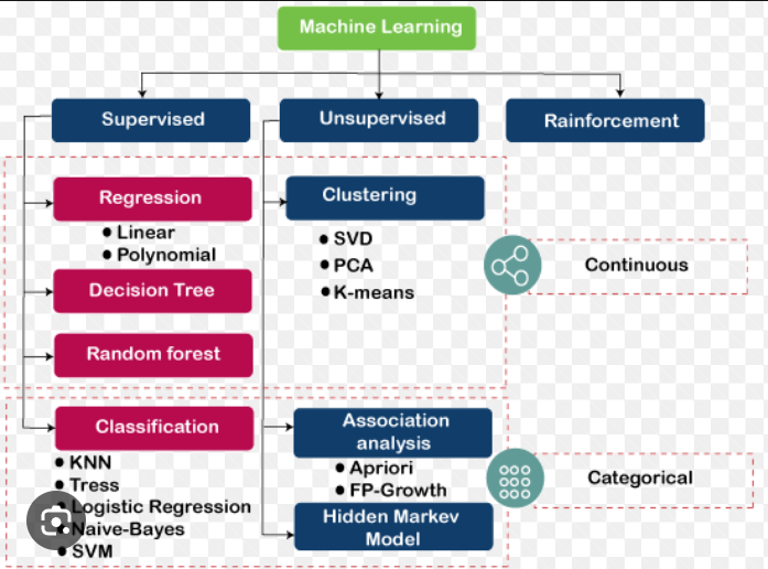
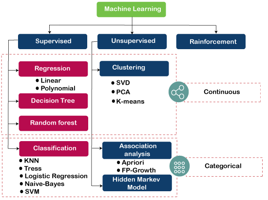
Machine Learning Algorithms: What are the types of Machine Learning Algorithms?

So, Machine Learning Algorithms can be categorized by the following three types.

Machine Learning Algorithms: What is Supervised Learning?

This category is termed as supervised learning because the process of an algorithm learning from the training dataset can be thought of as a teacher teaching his students. The algorithm continuously predicts the result on the basis of training data and is continuously corrected by the teacher. The learning continues until the algorithm achieves an acceptable level of performance.

Let me rephrase you this in simple terms:

In Supervised machine learning algorithm, every instance of the training dataset consists of input attributes and expected output. The training dataset can take any kind of data as input like values of a database row, the pixels of an image, or even an audio frequency histogram. 

Example: In Biometric Attendance you can train the machine with inputs of your biometric identity – it can be your thumb, iris or ear-lobe, etc. Once the machine is trained it can validate your future input and can easily identify you.

Machine Learning Algorithms: What is Unsupervised Learning? 

Well, this category of machine learning is known as unsupervised because unlike supervised learning there is no teacher. Algorithms are left on their own to discover and return the interesting structure in the data.

The goal for unsupervised learning is to model the underlying structure or distribution in the data in order to learn more about the data.

Let me rephrase it for you in simple terms:

In the unsupervised learning approach, the sample of a training dataset does not have an expected output associated with them. Using the unsupervised learning algorithms you can detect patterns based on the typical characteristics of the input data. Clustering can be considered as an example of a machine learning task that uses the unsupervised learning approach. The machine then groups similar data samples and identify different clusters within the data.

Example: Fraud Detection is probably the most popular use-case of Unsupervised Learning. Utilizing past historical data on fraudulent claims, it is possible to isolate new claims based on its proximity to clusters that indicate fraudulent patterns. 

Also, enroll in Artificial Intelligence and Machine Learning courses to become proficient in this AI and ML.

Machine Learning Algorithms: What is Reinforcement Learning?

Reinforcement learning can be thought of like a hit and trial method of learning. The machine gets a Reward or Penalty point for each action it performs. If the option is correct, the machine gains the reward point or gets a penalty point in case of a wrong response.

The reinforcement learning algorithm is all about the interaction between the environment and the learning agent. The learning agent is based on exploration and exploitation.

Exploration is when the learning agent acts on trial and error and Exploitation is when it performs an action based on the knowledge gained from the environment. The environment rewards the agent for every correct action, which is the reinforcement signal. With the aim of collecting more rewards obtained, the agent improves its environment knowledge to choose or perform the next action.

Let see how Pavlov trained his dog using reinforcement training?

Pavlov divided the training of his dog into three stages.

Stage 1: In the first part, Pavlov gave meat to the dog, and in response to the meat, the dog started salivating.

Stage 2: In the next stage he created a sound with a bell, but this time the dogs did not respond to anything.

Stage 3: In the third stage, he tried to train his dog by using the bell and then giving them food. Seeing the food the dog started salivating.

Eventually, the dogs started salivating just after hearing the bell, even if the food was not given as the dog was reinforced that whenever the master will ring the bell, he will get the food. Reinforcement Learning is a continuous process, either by stimulus or feedback.

Machine Learning Algorithms: List of Machine Learning Algorithms 

Here is the list of 5 most commonly used machine learning algorithms. 

1. Linear Regression
2. Logistic Regression
3. Decision Tree
4. Naive Bayes
5. kNN

1. Linear Regression

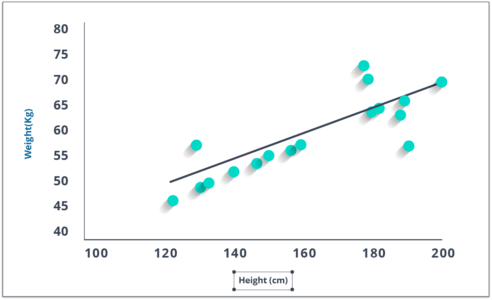
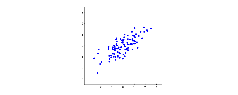
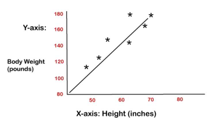
It is used to estimate real values (cost of houses, number of calls, total sales etc.) based on continuous variables. Here, we establish a relationship between the independent and dependent variables by fitting the best line. This best fit line is known as the regression line and represented by a linear equation Y= aX + b.

The best way to understand linear regression is to relive this experience of childhood. Let us say, you ask a child in fifth grade to arrange people in his class by increasing order of weight, without asking them their weights! What do you think the child will do? He/she would likely look (visually analyze) at the height and build of people and arrange them using a combination of these visible parameters. This is a linear regression in real life! The child has actually figured out that height and build would be correlated to the weight by a relationship, which looks like the equation above.

In this equation:

• Y – Dependent Variable
• a – Slope
• X – Independent variable
• b – Intercept

These coefficients a and b are derived based on minimizing the ‘sum of squared differences’ of distance between data points and regression line.

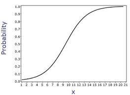
Look at the plot given. Here, we have identified the best fit having linear equation y=0.2811x+13.9. Now using this equation, we can find the weight, knowing the height of a person.

R-Code:

#Load Train and Test datasets
#Identify feature and response variable(s) and values must be numeric and numpy arrays
x_train <- input_variables_values_training_datasets
y_train <- target_variables_values_training_datasets
x_test <- input_variables_values_test_datasets
x <- cbind(x_train,y_train)
# Train the model using the training sets and check score
linear <- lm(y_train ~ ., data = x)
summary(linear)
#Predict Output
predicted= predict(linear,x_test) 

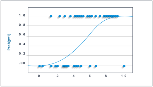
2. Logistic Regression

Don’t get confused by its name! It is a classification, and not a regression algorithm. It is used to estimate discrete values ( Binary values like 0/1, yes/no, true/false ) based on a given set of independent variable(s). In simple words, it predicts the probability of occurrence of an event by fitting data to a logit function. Hence, it is also known as logit regression. Since it predicts the probability, its output values lie between 0 and 1.

Again, let us try and understand this through a simple example.

Let’s say your friend gives you a puzzle to solve. There are only 2 outcome scenarios – either you solve it or you don’t. Now imagine, that you are being given a wide range of puzzles/quizzes in an attempt to understand which subjects you are good at. The outcome of this study would be something like this – if you are given a trigonometry based tenth-grade problem, you are 70% likely to solve it. On the other hand, if it is grade fifth history question, the probability of getting an answer is only 30%. This is what Logistic Regression provides you.

Coming to the math, the log odds of the outcome is modeled as a linear combination of the predictor variables.

odds= p/ (1-p) = probability of event occurrence / probability of not event occurrence ln(odds) = ln(p/(1-p)) logit(p) = ln(p/(1-p)) = b0+b1X1+b2X2+b3X3....+bkXk

Above, p is the probability of the presence of the characteristic of interest. It chooses parameters that maximize the likelihood of observing the sample values rather than that minimize the sum of squared errors (like in ordinary regression).

Now, you may ask, why take a log? For the sake of simplicity, let’s just say that this is one of the best mathematical ways to replicate a step function. I can go in more details, but that will beat the purpose of this blog.

R-Code:

x <- cbind(x_train,y_train)
# Train the model using the training sets and check score
logistic <- glm(y_train ~ ., data = x,family='binomial')
summary(logistic)
#Predict Output
predicted= predict(logistic,x_test)

There are many different steps that could be tried in order to improve the model:

• including interaction terms
• removing features
• regularization techniques
• using a non-linear model

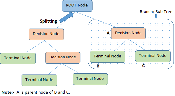
3. Decision Tree

Now, this is one of my favorite algorithms. It is a type of supervised learning algorithm that is mostly used for classification problems. Surprisingly, it works for both categorical and continuous dependent variables. In this algorithm, we split the population into two or more homogeneous sets. This is done based on the most significant attributes/ independent variables to make as distinct groups as possible.

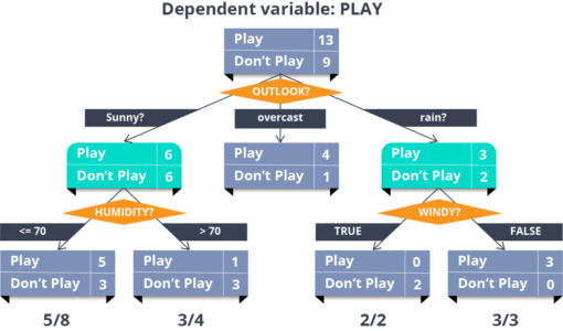
In the image above, you can see that population is classified into four different groups based on multiple attributes to identify ‘if they will play or not’. 

R-Code:

library(rpart)
x <- cbind(x_train,y_train)
# grow tree 
fit <- rpart(y_train ~ ., data = x,method="class")
summary(fit)
#Predict Output 
predicted= predict(fit,x_test)

4. Naive Bayes

This is a classification technique based on Bayes’ theorem with an assumption of independence between predictors. In simple terms, a Naive Bayes classifier assumes that the presence of a particular feature in a class is unrelated to the presence of any other feature.

For example, a fruit may be considered to be an apple if it is red, round, and about 3 inches in diameter. Even if these features depend on each other or upon the existence of the other features, a naive Bayes classifier would consider all of these properties to independently contribute to the probability that this fruit is an apple.

Naive Bayesian model is easy to build and particularly useful for very large data sets. Along with simplicity, Naive Bayes is known to outperform even highly sophisticated classification methods.

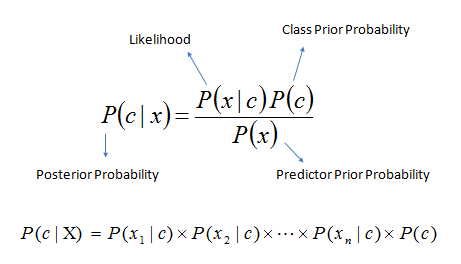
Bayes theorem provides a way of calculating posterior probability P(c|x) from P(c), P(x) and P(x|c). Look at the equation below:

Here,

• P(c|x) is the posterior probability of class (target) given predictor (attribute). 
• P(c) is the prior probability of class. 
• P(x|c) is the likelihood which is the probability of predictor given class. 
• P(x) is the prior probability of predictor.

Example: Let’s understand it using an example. Below I have a training data set of weather and corresponding target variable ‘Play’. Now, we need to classify whether players will play or not based on weather condition. Let’s follow the below steps to perform it.

Step 1: Convert the data set to the frequency table

Step 2: Create a Likelihood table by finding the probabilities like Overcast probability = 0.29 and probability of playing is 0.64.

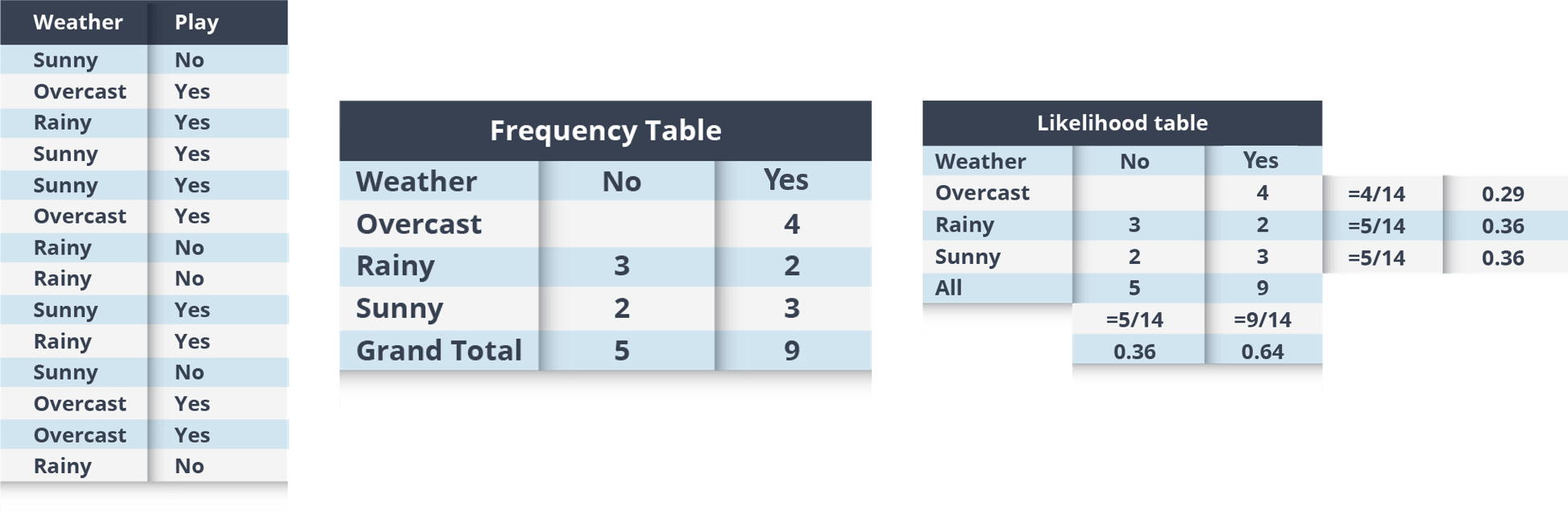
Step 3: Now, use the Naive Bayesian equation to calculate the posterior probability for each class. The class with the highest posterior probability is the outcome of prediction.

Problem: Players will pay if the weather is sunny, is this statement is correct?

We can solve it using above discussed method, so P(Yes | Sunny) = P( Sunny | Yes) * P(Yes) / P (Sunny)

Here we have P (Sunny |Yes) = 3/9 = 0.33, P(Sunny) = 5/14 = 0.36, P( Yes)= 9/14 = 0.64

Now, P (Yes | Sunny) = 0.33 * 0.64 / 0.36 = 0.60, which has higher probability.

Data Science with R Programming Certification Training Course

Weekday / Weekend BatchesSee Batch Details

Naive Bayes uses a similar method to predict the probability of different class based on various attributes. This algorithm is mostly used in text classification and with problems having multiple classes.

R-Code:

library(e1071)
x <- cbind(x_train,y_train)
# Fitting model
fit <-naiveBayes(y_train ~ ., data = x)
summary(fit)
#Predict Output 
predicted= predict(fit,x_test)

5. kNN (k- Nearest Neighbors)

It can be used for both classification and regression problems. However, it is more widely used in classification problems in the industry. K nearest neighbors is a simple algorithm that stores all available cases and classifies new cases by a majority vote of its k neighbors. The case being assigned to the class is most common amongst its K nearest neighbors measured by a distance function.

These distance functions can be Euclidean, Manhattan, Minkowski and Hamming distance. First three functions are used for continuous function and the fourth one (Hamming) for categorical variables. If K = 1, then the case is simply assigned to the class of its nearest neighbor. At times, choosing K turns out to be a challenge while performing kNN modeling.

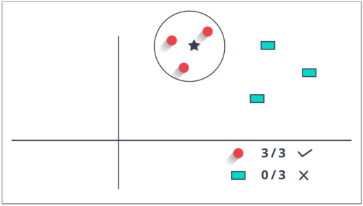
KNN can easily be mapped to our real lives. If you want to learn about a person, of whom you have no information, you might like to find out about his close friends and the circles he moves in and gain access to his/her information!

R-Code:

library(knn)
x <- cbind(x_train,y_train)
# Fitting model
fit <-knn(y_train ~ ., data = x,k=5)
summary(fit)
#Predict Output 
predicted= predict(fit,x_test)

Things to consider before selecting KNN:

• KNN is computationally expensive
• Variables should be normalized else higher range variables can bias it
• Works on pre-processing stage more before going for kNN like an outlier, noise removal

This brings me to the end of this blog. Stay tuned for more content on Machine Learning and Data Science!

Are you wondering how to advance once you know the basics of what Machine Learning is? Take a look at Edureka’s Machine Learning Certification, which will help you get on the right path to succeed in this fascinating field. Learn the fundamentals of Machine Learning, machine learning steps and methods that include unsupervised and supervised learning, mathematical and heuristic aspects, and hands-on modeling to create algorithms. You will be prepared for the position of Machine Learning engineer.

You can also take a Machine Learning Course Masters Program. The program will provide you with the most in-depth and practical information on machine-learning applications in real-world situations. Additionally, you’ll learn the essentials needed to be successful in the field of machine learning, such as statistical analysis, Python, and data science.

Machine learning (ML) is a type of algorithm that automatically improves itself based on experience, not by a programmer writing a better algorithm. The algorithm gains experience by processing more and more data and then modifying itself based on the properties of the data.

Types of machine learning

There are many varieties of machine learning techniques, but here are three general approaches:

• reinforcement learning: The algorithm performs actions that will be rewarded the most. Often used by game-playing AI or navigational robots.
• unsupervised machine learning: The algorithm finds patterns in unlabeled data by clustering and identifying similarities. Popular uses include recommendation systems and targeted advertising.
• supervised machine learning: The algorithm analyzes labeled data and learns how to map input data to an output label. Often used for classification and prediction.

Let’s dive into one of the most common approaches to understand more about how a machine learning algorithm works.

Neural networks

An increasingly popular approach to supervised machine learning is the neural network. A neural network operates similarly to how we think brains work, with input flowing through many layers of “neurons” and eventually leading to an output.

Diagram of a neural network, with circles representing each neuron and lines representing connections between neurons. The network starts on the left with a column of 3 neurons labeled “Input”. Those neurons are connected to another column of 4 neurons, which itself connects to another column of 4, and those neurons are labeled “Hidden layers”. The second hidden layer of neurons is connected to a column of 3 neurons labeled “Output”.

Training a network

Computer programmers don’t actually program each neuron. Instead, they train a neural network using a massive amount of labeled data.

The training data depends on the goal of the network. If its purpose is to classify images, a training data set could contain thousands of images labeled as “bird”, “airplane”, etc.

A grid of images in 10 categories (airplane, automobile, bird, cat, deer, dog, frog, horse, ship, truck).

Images from the CIFAR10 training data set. Image source: CIFAR10

The goal of the training phase is to determine weights for the connections between neurons that will correctly classify the training data.

A diagram of a neural network classifying an image of a plane. Parts of the image are fed into the first layer of neurons, those neurons lead to a middle layer, and those neurons lead to a final layer of neurons. Each edge between neurons is labeled with a question mark, denoting an unknown weight.

The weights between the neurons are unknown (labeled with a “?” here), and the neural network wants to find weights that will result in classifying each image correctly.

The neural network starts off with all the weights set to random values, so its initial classifications are way off. It learns from its mistakes, however, and eventually comes up with a set of weights that do the best job at classifying all of the training data.

A diagram of a neural network classifying an image of a plane. Parts of the image are fed into the first layer of neurons, those neurons lead to a middle layer, and those neurons lead to a final layer of neurons. Each neuron has a weight (from 0 to 1). In the final layer, the neuron labeled “plane” has the highest weight.

Each of the connections between neurons is assigned a weight (represented by shades of green). A neuron multiplies each connection weight by the value of the input neuron, and sums up all of those to come up with a single number (shown on each neuron). The neuron will only send its value to the next layer if it’s above a threshold.

Using the network

When the neural network is asked to classify an image, it uses the learned weights and outputs the possible classes and their probabilities.

Diagram of a neural network, with circles representing each neuron and lines representing connections between neurons. The network starts on the left with an image of a fox. The image is broken into 4 parts, and those parts are connected to column of 4 neurons, which itself connects to another column of 4. The second column is connected to 3 possible outputs: “Fox (0.85)”, “Dog (0.65)”, and “Cat (0.25)”.

Accuracy

The accuracy of a neural network is highly dependent on its training data, both the amount and diversity. Has the network seen the object from multiple angles and lighting conditions? Has it seen the object against many different backgrounds? Has it really seen all varieties of that object? If we want a neural network to truly understand the world, we need to expose it to the huge diversity of our world.

Companies, governments, and institutions are increasingly using machine learning to make decisions for them. They often call it “artificial intelligence,” but a machine learning algorithm is only as intelligent as its training data. If the training data is biased, then the algorithm is biased. And unfortunately, training data is biased more often than it’s not.

In the following articles, we’ll explore the ramifications of letting machines make decisions for us based on biased data.

Some Basic Machine Learning Algorithms

elow you’ll find descriptions of and links to some basic and powerful machine-learning algorithms, including:

• Attention Mechanisms & Memory Networks
• Bayes Theorem & Naive Bayes Classifiers
• Decision Trees
• Eigenvectors, Eigenvalues and Machine Learning
• Evolutionary & Genetic Algorithms
• Expert Systems/Rules Engines/Symbolic Reasoning
• Generative Adversarial Networks (GANs)
• Graph Analytics and ML
• Linear Regression
• Logistic Regression
• LSTMs and Recurrent Neural Networks
• Markov Chain Monte Carlo Methods (MCMC)
• Neural Networks
• Random Forests
• Reinforcement Learning
• Word2vec, Neural Embeddings and NLP

Machine learning algorithms are programs (math and logic) that adjust themselves to perform better as they are exposed to more data. The “learning” part of machine learning means that those programs change how they process data over time, much as humans change how they process data by learning. So a machine-learning algorithm is a program with a specific way to adjusting its own parameters, given feedback on its previous performance in making predictions about a dataset.

Linear Regression

Linear regression is simple, which makes it a great place to start thinking about algorithms more generally. Here it is:

ŷ = a * x + b

Read aloud, you’d say “y-hat equals a times x plus b.”

• y-hat is the output, or guess made by the algorithm, the dependent variable.
• a is the coefficient. It’s also the slope of the line that expresses the relationship between x and y-hat.
• x is the input, the given or independent variable.
• b is the intercept, where the line crosses the y axis.

Linear regression expresses a linear relationship between the input x and the output y; that is, for every change in x, y-hat will change by the same amount no matter how far along the line you are. The x is transformed by the same a and b at every point.

Linear regression with only one input variable is called Simple Linear Regression. With more than one input variable, it is called Multiple Linear Regression. An example of Simple Linear Regression would be attempting to predict a house price based on the square footage of the house and nothing more.

house_price_estimate = a * square_footage + b

Multiple Linear Regression would take other variables into account, such as the distance between the house and a good public school, the age of the house, etc.

The reason why we’re dealing with y-hat, an estimate about the real value of y, is because linear regression is a formula used to estimate real values, and error is inevitable. Linear regression is often used to “fit” a scatter plot of given x-y pairs. A good fit minimizes the error between y-hat and the actual y; that is, choosing the right a and b will minimize the sum of the differences between each y and its respective y-hat.

That scatter plot of data points may look like a baguette – long in one direction and short in another – in which case linear regression may achieve a fit. (If the data points look like a meandering river, a straight line is probably not the right function to use to make predictions.)

Testing one line after another against the data points of the scatter plot, and automatically correcting it in order to minimize the sum of differences between the line and the points, could be thought of as machine learning in its simplest form.

Apply AI to Business Simulations »

Logistic Regression

Let’s analyze the name first. Logistic regression is not really regression, not in the sense of linear regression, which predicts continuous numerical values. (And it has nothing to do with logistics. 😉

Logistic regression does not do that. It’s actually a binomial classifier that acts like a light switch. A light switch essentially has two states, on and off. Logistic regression takes input data and classifies it as category or not_category, on or off expressed as 1 or 0, based on the strength of the input’s signal. So it’s a light switch for signal that you find in the data. If you want to mix the metaphor, it’s actually more like a transistor, since it both amplifies and gates the signal. More on that here.

Logistic regression takes input data and squishes it, so that no matter what the range of the input is, it will be compressed into the space between 1 and 0. Notice, in the image below, no matter how large the input x becomes, the output y cannot exceed 1, which it asymptotically approaches, and no matter low x is, y cannot fall below 0. That’s how logistic regression compresses input data into a range between 0 and 1, through this s-shaped, sigmoidal transform.

Decision Tree

Decision, or decide, stems from the Latin decidere, which itself is the combination of “de” (off) and “caedere” (to cut). So decision is about the cutting off of possibilities. Decision trees can be used to classify data, and they cut off possibilities of what a given instance of data might be by examining a data point’s features. Is it bigger than a bread box? Well, then it’s not a marble. Is it alive? Well, then it’s not a bicycle. Think of a decision as a game of 20 questions that an algorithm is asking about the data point under examination.

A decision tree is a series of nodes, a directional graph that starts at the base with a single node and extends to the many leaf nodes that represent the categories that the tree can classify. Another way to think of a decision tree is as a flow chart, where the flow starts at the root node and ends with a decision made at the leaves. It is a decision-support tool. It uses a tree-like graph to show the predictions that result from a series of feature-based splits.

Here are some useful terms for describing a decision tree:

• Root Node: A root node is at the beginning of a tree. It represents entire population being analyzed. From the root node, the population is divided according to various features, and those sub-groups are split in turn at each decision node under the root node.
• Splitting: It is a process of dividing a node into two or more sub-nodes.
• Decision Node: When a sub-node splits into further sub-nodes, it’s a decision node.
• Leaf Node or Terminal Node: Nodes that do not split are called leaf or terminal nodes.
• Pruning: Removing the sub-nodes of a parent node is called pruning. A tree is grown through splitting and shrunk through pruning.
• Branch or Sub-Tree: A sub-section of decision tree is called branch or a sub-tree, just as a portion of a graph is called a sub-graph.
• Parent Node and Child Node: These are relative terms. Any node that falls under another node is a child node or sub-node, and any node which precedes those child nodes is called a parent node.

Decision trees are a popular algorithm for several reasons:

• Explanatory Power: The output of decision trees is interpretable. It can be understood by people without analytical or mathematical backgrounds. It does not require any statistical knowledge to interpret them.
• Exploratory data analysis: Decision trees can enable analysts to identify significant variables and important relations between two or more variables, helping to surface the signal contained by many input variables.
• Minimal data cleaning: Because decision trees are resilient to outliers and missing values, they require less data cleaning than some other algorithms.
• Any data type: Decision trees can make classifications based on both numerical and categorical variables.
• Non-parametric: A decision tree is a non-parametric algorithm, as opposed to neural networks, which process input data transformed into a tensor, via tensor multiplication using large number of coefficients, known as parameters.

Disadvantages

• Overfitting: Over fitting is a common flaw of decision trees. Setting constraints on model parameters and making the model simpler through pruning are two ways to regularize a decision tree.
• Predicting continuous variables: While decision trees can ingest continuous numerical input, they are not a practical way to predict such values, since decision-tree predictions must be separated into discrete categories, which results in a loss of information when applying the model to continuous values.
• Heavy feature engineering: The flip side of a decision tree’s explanatory power is that it requires heavy feature engineering. When dealing with unstructured data or data with latent factors, this makes decision trees sub-optimal. Neural networks are clearly superior in this regard.

Random Forest

Random forests are made of many decision trees. They are ensembles of decision trees, each decision tree created by using a subset of the attributes used to classify a given population (they are sub-trees, see above). Those decision trees vote on how to classify a given instance of input data, and the random forest bootstraps those votes to choose the best prediction. This is done to prevent overfitting, a common flaw of decision trees.

A random forest is a supervised classification algorithm. It creates a forest (many decision trees) and orders their nodes and splits randomly. The more trees in the forest, the better the results it can produce.

If you input a training dataset with targets and features into the decision tree, it will formulate some set of rules that can be used to perform predictions.

Example: You want to predict whether a visitor to your e-commerce Web site will enjoy a mystery novel. First, collect information about past books they’ve read and liked. Metadata about the novels will be the input; e.g. number of pages, author, publication date, which series it’s part of if any. The decision tree contains rules that apply to those features; for example, some readers like very long books and some don’t. Inputting metadata about new novels will result in a prediction regarding whether or not the Web site visitor in question would like that novel. Arranging the nodes and defining the rules relies on information gain and Gini-index calculations. With random forests, finding the root node and splitting the feature nodes is done randomly.

What are Machine Learning Algorithms for AI?

Machine learning (ML) algorithms are computer programs that adapt and evolve based on the data they process to produce predetermined outcomes. They are essentially mathematical models that “learn” by being fed data—often referred to as “training data.” Common types of ML algorithms include linear regression and decision trees. Practical applications of ML algorithms include fraud detection and the automatic delivery of personalized marketing offers in retail.

Broadly speaking, there are two main categories of ML algorithms: supervised and unsupervised ML. Supervised ML algorithms involve “teaching” the machine to produce outputs based on its training data, which is already labelled or structured. Unsupervised ML algorithms, on the other hand, work with unstructured data—data that hasn’t already been classified or labeled.

Why Do Machine Learning Algorithms Matter?

ML is the most widely used and fastest-growing subset of AI today. Used to improve a wide array of computing concepts, including computer programming itself, it is often referred to as Software 2.0.

ML algorithms are integrated into just about every kind of device and hardware, from smartphones to servers to watches and sensors. They are increasingly the backbone behind many technological innovations and benefits, from ridesharing to autonomous vehicles to spam filtering, and many more.

Machine Learning algorithms are the programs that can learn the hidden patterns from the data, predict the output, and improve the performance from experiences on their own. Different algorithms can be used in machine learning for different tasks, such as simple linear regression that can be used for prediction problems like stock market prediction, and the KNN algorithm can be used for classification problems.

In this topic, we will see the overview of some popular and most commonly used machine learning algorithms along with their use cases and categories.

Types of Machine Learning Algorithms

Machine Learning Algorithm can be broadly classified into three types:

1. Supervised Learning Algorithms
2. Unsupervised Learning Algorithms
3. Reinforcement Learning algorithm

The below diagram illustrates the different ML algorithm, along with the categories:

1) Supervised Learning Algorithm

Supervised learning is a type of Machine learning in which the machine needs external supervision to learn. The supervised learning models are trained using the labeled dataset. Once the training and processing are done, the model is tested by providing a sample test data to check whether it predicts the correct output.

The goal of supervised learning is to map input data with the output data. Supervised learning is based on supervision, and it is the same as when a student learns things in the teacher’s supervision. The example of supervised learning is spam filtering.

Supervised learning can be divided further into two categories of problem:

• Classification
• Regression

Examples of some popular supervised learning algorithms are Simple Linear regression, Decision Tree, Logistic Regression, KNN algorithm, etc. 

2) Unsupervised Learning Algorithm

It is a type of machine learning in which the machine does not need any external supervision to learn from the data, hence called unsupervised learning. The unsupervised models can be trained using the unlabelled dataset that is not classified, nor categorized, and the algorithm needs to act on that data without any supervision. In unsupervised learning, the model doesn’t have a predefined output, and it tries to find useful insights from the huge amount of data. These are used to solve the Association and Clustering problems. Hence further, it can be classified into two types:

• Clustering
• Association

Examples of some Unsupervised learning algorithms are K-means Clustering, Apriori Algorithm, Eclat, etc. 

3) Reinforcement Learning

In Reinforcement learning, an agent interacts with its environment by producing actions, and learn with the help of feedback. The feedback is given to the agent in the form of rewards, such as for each good action, he gets a positive reward, and for each bad action, he gets a negative reward. There is no supervision provided to the agent. Q-Learning algorithm is used in reinforcement learning. 

List of Popular Machine Learning Algorithm

1. Linear Regression Algorithm
2. Logistic Regression Algorithm
3. Decision Tree
4. SVM
5. Naïve Bayes
6. KNN
7. K-Means Clustering
8. Random Forest
9. Apriori
10. PCA

1. Linear Regression

Linear regression is one of the most popular and simple machine learning algorithms that is used for predictive analysis. Here, predictive analysis defines prediction of something, and linear regression makes predictions for continuous numbers such as salary, age, etc.

It shows the linear relationship between the dependent and independent variables, and shows how the dependent variable(y) changes according to the independent variable (x).

It tries to best fit a line between the dependent and independent variables, and this best fit line is knowns as the regression line.

The equation for the regression line is:

y= a₀+ a*x+ b

Here, y= dependent variable

x= independent variable

a₀ = Intercept of line.

Linear regression is further divided into two types:

• Simple Linear Regression: In simple linear regression, a single independent variable is used to predict the value of the dependent variable.
• Multiple Linear Regression: In multiple linear regression, more than one independent variables are used to predict the value of the dependent variable.

2. Logistic Regression

Logistic regression is the supervised learning algorithm, which is used to predict the categorical variables or discrete values. It can be used for the classification problems in machine learning, and the output of the logistic regression algorithm can be either Yes or NO, 0 or 1, Red or Blue, etc.

Logistic regression is similar to the linear regression except how they are used, such as Linear regression is used to solve the regression problem and predict continuous values, whereas Logistic regression is used to solve the Classification problem and used to predict the discrete values.

Instead of fitting the best fit line, it forms an S-shaped curve that lies between 0 and 1. The S-shaped curve is also known as a logistic function that uses the concept of the threshold. Any value above the threshold will tend to 1, and below the threshold will tend to 0.

3. Decision Tree Algorithm

A decision tree is a supervised learning algorithm that is mainly used to solve the classification problems but can also be used for solving the regression problems. It can work with both categorical variables and continuous variables. It shows a tree-like structure that includes nodes and branches, and starts with the root node that expand on further branches till the leaf node. The internal node is used to represent the features of the dataset, branches show the decision rules, and leaf nodes represent the outcome of the problem.

Some real-world applications of decision tree algorithms are identification between cancerous and non-cancerous cells, suggestions to customers to buy a car, etc.

4. Support Vector Machine Algorithm

A support vector machine or SVM is a supervised learning algorithm that can also be used for classification and regression problems. However, it is primarily used for classification problems. The goal of SVM is to create a hyperplane or decision boundary that can segregate datasets into different classes.

The data points that help to define the hyperplane are known as support vectors, and hence it is named as support vector machine algorithm.

Some real-life applications of SVM are face detection, image classification, Drug discovery, etc. Consider the below diagram:

As we can see in the above diagram, the hyperplane has classified datasets into two different classes.

5. Naïve Bayes Algorithm:

Naïve Bayes classifier is a supervised learning algorithm, which is used to make predictions based on the probability of the object. The algorithm named as Naïve Bayes as it is based on Bayes theorem, and follows the naïve assumption that says’ variables are independent of each other.

The Bayes theorem is based on the conditional probability; it means the likelihood that event(A) will happen, when it is given that event(B) has already happened. The equation for Bayes theorem is given as:

Naïve Bayes classifier is one of the best classifiers that provide a good result for a given problem. It is easy to build a naïve bayesian model, and well suited for the huge amount of dataset. It is mostly used for text classification. 

6. K-Nearest Neighbour (KNN)

K-Nearest Neighbour is a supervised learning algorithm that can be used for both classification and regression problems. This algorithm works by assuming the similarities between the new data point and available data points. Based on these similarities, the new data points are put in the most similar categories. It is also known as the lazy learner algorithm as it stores all the available datasets and classifies each new case with the help of K-neighbours. The new case is assigned to the nearest class with most similarities, and any distance function measures the distance between the data points. The distance function can be Euclidean, Minkowski, Manhattan, or Hamming distance, based on the requirement. 

7. K-Means Clustering

K-means clustering is one of the simplest unsupervised learning algorithms, which is used to solve the clustering problems. The datasets are grouped into K different clusters based on similarities and dissimilarities, it means, datasets with most of the commonalties remain in one cluster which has very less or no commonalities between other clusters. In K-means, K-refers to the number of clusters, and means refer to the averaging the dataset in order to find the centroid.

It is a centroid-based algorithm, and each cluster is associated with a centroid. This algorithm aims to reduce the distance between the data points and their centroids within a cluster.

This algorithm starts with a group of randomly selected centroids that form the clusters at starting and then perform the iterative process to optimize these centroids’ positions.

It can be used for spam detection and filtering, identification of fake news, etc.

8. Random Forest Algorithm

Random forest is the supervised learning algorithm that can be used for both classification and regression problems in machine learning. It is an ensemble learning technique that provides the predictions by combining the multiple classifiers and improve the performance of the model.

It contains multiple decision trees for subsets of the given dataset, and find the average to improve the predictive accuracy of the model. A random-forest should contain 64-128 trees. The greater number of trees leads to higher accuracy of the algorithm.

To classify a new dataset or object, each tree gives the classification result and based on the majority votes, the algorithm predicts the final output.

Random forest is a fast algorithm, and can efficiently deal with the missing & incorrect data. 

9. Apriori Algorithm

Apriori algorithm is the unsupervised learning algorithm that is used to solve the association problems. It uses frequent itemsets to generate association rules, and it is designed to work on the databases that contain transactions. With the help of these association rule, it determines how strongly or how weakly two objects are connected to each other. This algorithm uses a breadth-first search and Hash Tree to calculate the itemset efficiently.

The algorithm process iteratively for finding the frequent itemsets from the large dataset.

The apriori algorithm was given by the R. Agrawal and Srikant in the year 1994. It is mainly used for market basket analysis and helps to understand the products that can be bought together. It can also be used in the healthcare field to find drug reactions in patients. 

10. Principle Component Analysis

Principle Component Analysis (PCA) is an unsupervised learning technique, which is used for dimensionality reduction. It helps in reducing the dimensionality of the dataset that contains many features correlated with each other. It is a statistical process that converts the observations of correlated features into a set of linearly uncorrelated features with the help of orthogonal transformation. It is one of the popular tools that is used for exploratory data analysis and predictive modeling.

PCA works by considering the variance of each attribute because the high variance shows the good split between the classes, and hence it reduces the dimensionality.

Some real-world applications of PCA are image processing, movie recommendation system, optimizing the power allocation in various communication channels.

What are machine learning algorithms?

Machine learning algorithms are pieces of code that help people explore, analyze, and find meaning in complex data sets. Each algorithm is a finite set of unambiguous step-by-step instructions that a machine can follow to achieve a certain goal. In a machine learning model, the goal is to establish or discover patterns that people can use to make predictions or categorize information. What is machine learning?

Machine learning algorithms use parameters that are based on training data—a subset of data that represents the larger set. As the training data expands to represent the world more realistically, the algorithm calculates more accurate results.

Different algorithms analyze data in different ways. They’re often grouped by the machine learning techniques that they’re used for: supervised learning, unsupervised learning, and reinforcement learning. The most commonly used algorithms use regression and classification to predict target categories, find unusual data points, predict values, and discover similarities.

Machine learning techniques

As you learn more about machine learning algorithms, you’ll find that they typically fall within one of three machine learning techniques:

Supervised learning

In supervised learning, algorithms make predictions based on a set of labeled examples that you provide. This technique is useful when you know what the outcome should look like.
 

For example, you provide a dataset that includes city populations by year for the past 100 years, and you want to know what the population of a specific city will be four years from now. The outcome uses labels that already exist in the data set: population, city, and year.
 

Unsupervised learning

In unsupervised learning, the data points aren’t labeled—the algorithm labels them for you by organizing the data or describing its structure. This technique is useful when you don’t know what the outcome should look like.

For example, you provide customer data, and you want to create segments of customers who like similar products. The data that you’re providing isn’t labeled, and the labels in the outcome are generated based on the similarities that were discovered between data points.

Reinforcement learning

Reinforcement learning uses algorithms that learn from outcomes and decide which action to take next. After each action, the algorithm receives feedback that helps it determine whether the choice it made was correct, neutral, or incorrect. It’s a good technique to use for automated systems that have to make a lot of small decisions without human guidance.

For example, you’re designing an autonomous car, and you want to ensure that it’s obeying the law and keeping people safe. As the car gains experience and a history of reinforcement, it learns how to stay in its lane, go the speed limit, and brake for pedestrians.

What you can do with machine learning algorithms

Machine learning algorithms help you answer questions that are too complex to answer through manual analysis. There are many different machine learning algorithm types, but use cases for machine learning algorithms typically fall into one of these categories.

Predict a target category

Two-class (binary) classification algorithms divide the data into two categories. They’re useful for questions that have only two possible answers that are mutually exclusive, including yes/no questions. For example:

• Will this tire fail in the next 1,000 miles: yes or no?
• Which brings in more referrals: a $10 credit or a 15% discount?

Multiclass (multinomial) classification algorithms divide the data into three or more categories. They’re useful for questions that have three or more possible answers that are mutually exclusive. For example:

• In which month do the majority of travelers purchase airline tickets?
• What emotion is the person in this photo displaying?

Find unusual data points

Anomaly detection algorithms identify data points that fall outside of the defined parameters for what’s “normal.” For example, you would use anomaly detection algorithms to answer questions like:

• Where are the defective parts in this batch?
• Which credit card purchases might be fraudulent?

Predict values

Regression algorithms predict the value of a new data point based on historical data. They help you answer questions like:

• How much will the average two-bedroom home cost in my city next year?
• How many patients will come through the clinic on Tuesday?

See how values change over time

Time series algorithms show how a given value changes over time. With time series analysis and time series forecasting, data is collected at regular intervals over time and used to make predictions and identify trends, seasonality, cyclicity, and irregularity. Time series algorithms are used to answer questions like:

• Is the price of a given stock likely to rise or fall in the coming year?
• What will my expenses be next year?

Discover similarities

Clustering algorithms divide the data into multiple groups by determining the level of similarity between data points. Clustering algorithms work well for questions like:

• Which viewers like the same types of movies?
• Which printer models fail in the same way?

Classification

Classification algorithms use predictive calculations to assign data to preset categories. Classification algorithms are trained on input data, and used to answer questions like:

• Is this email spam?
• What is the sentiment (positive, negative, or neutral) of a given text?

Linear regression algorithms show or predict the relationship between two variable or factors by fitting a continuous straight line to the data. The line is often calculated using the Squared Error Cost function. Linear regression is one of the most popular types of regression analysis.

Logistic regression algorithms fit a continuous S-shaped curve to the data. Logistic regression is another popular type of regression analysis.

Naïve Bayes algorithms calculate the probability that an event will occur, based on the occurrence of a related event.

Support Vector Machines draw a hyperplane between the two closest data points. This marginalizes the classes and maximizes the distances between them to more clearly differentiate them.

Decision tree algorithms split the data into two or more homogeneous sets. They use if–then rules to separate the data based on the most significant differentiator between data points.

K-Nearest neighbor algorithms store all available data points and classify each new data point based on the data points that are closest to it, as measured by a distance function.

Random forest algorithms are based on decision trees, but instead of creating one tree, they create a forest of trees and then randomize the trees in that forest. Then, they aggregate votes from different random formations of the decision trees to determine the final class of the test object.

Gradient boosting algorithms produce a prediction model that bundles weak prediction models—typically decision trees—through an ensembling process that improves the overall performance of the model.

K-Means algorithms classify data into clusters—where K equals the number of clusters. The data points inside of each cluster are homogeneous, and they’re heterogeneous to data points in other clusters.

What are machine learning libraries?

A machine learning library is a set of functions, frameworks, modules, and routines written in a given language. Developers use the code in machine learning libraries as building blocks for creating machine learning solutions that can perform complex tasks. Instead of having to manually code every algorithm and formula in a machine learning solution, developers can find the functions and modules they need in one of many available ML libraries, and use those to build a solution that meets their needs.