If you are learning machine learning for getting a high profile data science job then you can’t miss out learning these 11 best machine learning algorithms.
Here, we will first go through supervised learning algorithms and then discuss about the unsupervised learning ones. While there are many more algorithms that are present in the arsenal of machine learning, our focus will be on the most popular machine learning algorithms.
These ML algorithms are quite essential for developing predictive modeling and for carrying out classification and prediction. These ML algorithms are the most useful for carrying out prediction and classification in both supervised as well as unsupervised scenarios.
Top Machine Learning Algorithms
Below are some of the best machine learning algorithms –
- Linear Regression
- Logistic Regression
- Decision Trees
- Naive Bayes
- Artificial Neural Networks
- K-means Clustering
- Anomaly Detection
- Gaussian Mixture Model
- Principal Component Analysis
- KNN
- Support Vector Machines
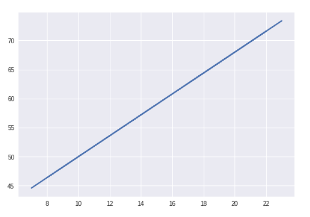
1. Linear Regression
The methodology for measuring the relationship between the two continuous variables is known as Linear regression. It comprises of two variables –
- Independent Variable – “x”
- Dependent Variable – “y”
In a simple linear regression, the predictor value is an independent value that does not have any underlying dependency on any variable. The relationship between x and y is described as follows –
y = mx + c
Here, m is the slope and c is the intercept.
Based on this equation, we can calculate the output that will be through the relationship exhibited between the dependent and the independent variable.
Learn linear regression in detail with DataFlair
2. Logistic Regression
This is the most popular ML algorithm for binary classification of the data-points. With the help of logistic regression, we obtain a categorical classification that results in the output belonging to one of the two classes. For example, predicting whether the price of oil would increase or not based on several predictor variables is an example of logistic regression.
Logistic Regression has two components – Hypothesis and Sigmoid Curve. Based on this hypothesis, one can derive the resultant likelihood of the event. Data obtained from the hypothesis is then fit into the log function that forms the S-shaped curve called ‘sigmoid’. Through this log function, one can determine the category to which the output data belongs to.
The sigmoid S-shaped curve is visualized as follows –
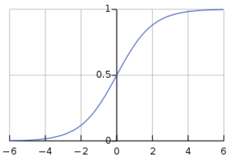
The above-generated graph is a result of this logistic equation –
1 / (1 + e^-x)
In the above equation, e is the base of the natural log and the S-shaped curve that we obtain is between 0 and 1. We write the equation for logistic regression as follows –
y = e^(b0 + b1*x) / (1 + e^(b0 + b1*x))
b0 and b1 are the two coefficients of the input x. We estimate these coefficients using the maximum likelihood function.
3. Decision Trees
Decision Trees facilitate prediction as well as classification. Using the decision trees, one can make decisions with a given set of input. Let us understand decision trees with the following example –
Let us assume that you want to go to the market to purchase a shampoo. First, you will analyze if you really do require shampoo. If you run out of it, then you will have to buy it from the market. Furthermore, you will look outside and assess the weather. That is, if it is raining, then you will not go and if it is not, you will. We can visualize this scenario intuitively with the following visualization.
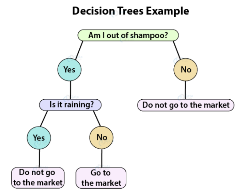
With the same principle, we can construct a hierarchical tree to obtain our output through several decisions. There are two procedures towards building a decision tree – Induction and Pruning. In Induction, we build the decision tree and in pruning, we simplify the tree by removing several complexities.
4. Naive Bayes
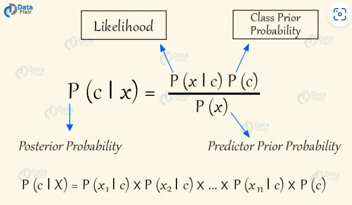
Naive Bayes are a class of conditional probability classifiers that are based on the Bayes Theorem. They assume independence of assumptions between the features.
Bayes Theorem lays down a standard methodology for the calculation of posterior probability P(c|x), from P(c), P(x), and P(x|c). In a Naive Bayes classifier, there is an assumption that the effect of the values of the predictor on a given class(c) is independent of other predictor values.
Bayes Theorem has many advantages. They can be easily implemented. Furthermore, Naive Bayes requires a small amount of training data and the results are generally accurate.
5. Artificial Neural Networks
Artificial Neural Networks share the same basic principle as the neurons in our nervous system. It comprises of neurons that act as units stacked in layers that propagate information from input layer to the final output layer. These Neural Networks have an input layer, hidden layer and a final output layer. There can be a single layered Neural Network (Perceptron) or a multi-layered neural network.
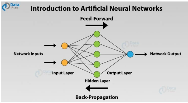
In this diagram, there is a single input layer that takes the input which is in the form of an output. Afterwards, the input is passed to the hidden layer that performs several mathematical functions to perform computation to get the desired output. For example, given an image of cats and dogs, the hidden layers compute maximum probability of the category to which our image belongs. This is an example of binary classification in which the cat or dog is assigned an appropriate place.
6. K-Means Clustering
K-means clustering is an iterative machine learning algorithm that performs partitioning of the data consisting of n values into subsequent k subgroups. Each of the n values with the nearest mean belongs to the k cluster.
Given a group of objects, we perform partitioning of the group into several sub-groups. The sub-groups have a similar basis where the distance of each data point in the sub-group has a meaning related to their centroids. It is the most popular form of unsupervised machine learning algorithm as it is quite easy to comprehend and implement.
The main objective of a K-means clustering algorithm is to reduce the Euclidean Distance to its minimum. This distance is the intra-cluster variance which we minimize using the following squared error function –
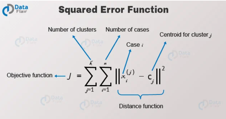
Here, J is the objective function of the centroid of the required cluster. There are K clusters and n are the number of cases in it. There are C centroids and j are the number of clusters.We determine the Euclidean Distance from the X data-point. Let us now look at some of the important algorithms for K-means clustering –
- In the first step, we initialize and select the k-points. These k-points denote the means.
- Using the Euclidean Distance, we find the data points that lie closest to the center of the cluster.
- We then proceed to calculate the mean of all the points which will help us to find the centroid.
- We perform iterative repeat of steps 1,2 and 3 until we have all the points assigned to the right cluster.
7. Anomaly Detection
In Anomaly Detection, we apply a technique to identify unusual patterns that are similar to the general pattern. These anomalous patterns or data points are known as outliers. The detection of these outliers is a crucial goal for many businesses that require intrusion detection, fraud detection, health system monitoring as well as fault detection in the operating environments.
Outlier is a rare occurring phenomena. It is an observation that is very different from the others. This could be due to some variability in measurement or simply the form of an error.
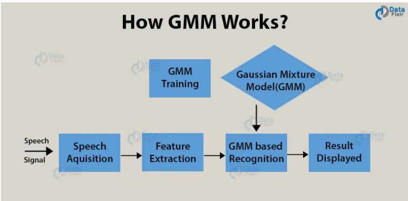
8. Gaussian Mixture Model
For representing a normally distributed subpopulation within an overall population, Gaussian Mixture Model is used. It does not require the data associated with the subpopulation. Therefore, the model is able to learn subpopulations automatically. As the assignment of the population is unclear, it comes under the category of unsupervised learning.
For example, assume that you have to create a model of the human height data. The mean height of males in male distribution is 5’8’’ and for females, it is 5’4’’. We are only aware of the height data and not the gender assignment. Distribution follows the sum of two scaled and two shifted normal distributions. We make this assumption with the help of the Gaussian Mixture Model or GMM. GMM can also have multiple components.
Using GMMs, we can extract important features from the speech data, we can also perform tracking of the objects in cases that have a number of mixture components and also the means that provide a prediction of the location of objects in a video sequence.
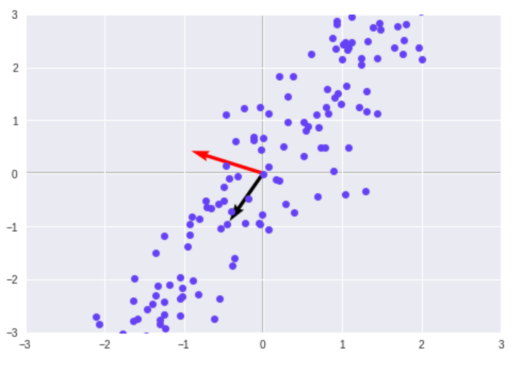
9. Principal Component Analysis
Dimensionality reduction is one of the most important concepts of Machine Learning. A data can have multiple dimensions. Let these dimensions be n. For instance, let there be a data scientist working on financial data which includes credit score, personal details, salary of the personnel and much more. For understanding significant labels contributing towards our model, we use dimensionality reduction. PCA is one of the most popular algorithms for reducing the dimensions.
Using PCA, one can reduce the number of dimensions while preserving the important features in our model. The PCAs are based on the number of dimensions and each PCA is perpendicular to the other. The dot product of all of the perpendicular PCAs is 0.
10. KNN
KNN is one of the many supervised machine learning algorithms that we use for data mining as well as machine learning. Based on the similar data, this classifier then learns the patterns present within. It is a non-parametric and a lazy learning algorithm. By non-parametric, we mean that the assumption for underlying data distribution does not hold valid. In lazy loading, there is no requirement for training data points for generating models.
The training data is utilized in testing phase causing the testing phase slower and costlier as compared with the training phase.
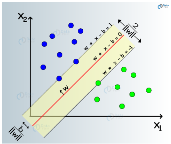
11. Support Vector Machines (SVM)
Support Vector Machines are a type of supervised machine learning algorithms that facilitate modeling for data analysis through regression and classification. SVMs are used mostly for classification. In SVM, we plot our data in an n-dimensional space. The value of each feature in SVM is same as that of specific coordinate. Then, we proceed to find the ideal hyperplane differentiating between the two classes.
Support Vectors represent the coordinate representation of individual observation. Therefore, it is a frontier method that we utilize for segregating the two classes.
Conclusion
In this article, we went through a number of machine learning algorithms that are essential in the data science industry. We studied a mix of supervised as well as unsupervised learning algorithms that are quite essential for the implementation of machine learning models. So, now you are ready to apply these ML algorithms concepts in your next data science job.