Machine learning (ML) is rapidly changing the world, from diverse types of applications and research pursued in industry and academia. Machine learning is affecting every part of our daily lives. From voice assistants using NLP and machine learning to make appointments, check our calendar, and play music, to programmatic advertisements — that are so accurate that they can predict what we will need before we even think of it.

More often than not, the complexity of the scientific field of machine learning can be overwhelming, making keeping up with “what is important” a very challenging task. However, to make sure that we provide a learning path to those who seek to learn machine learning, but are new to these concepts. In this article, we look at the most critical basic algorithms that hopefully make your machine learning journey less challenging.

Any suggestions or feedback is crucial to continue to improve. Please let us know in the comments if you have any.

Index

• Introduction to Machine Learning.
• Major Machine Learning Algorithms.
• Supervised vs. Unsupervised Learning.
• Linear Regression.
• Multivariable Linear Regression.
• Polynomial Regression.
• Exponential Regression.
• Sinusoidal Regression.
• Logarithmic Regression.

What is machine learning?

A computer program is said to learn from experience E with respect to some class of tasks T and performance measure P, if its performance at tasks in T, as measured by P, improves with experience E. ~ Tom M. Mitchell [1]

Machine learning behaves similarly to the growth of a child. As a child grows, her experience E in performing task T increases, which results in higher performance measure (P).

For instance, we give a “shape sorting block” toy to a child. (Now we all know that in this toy, we have different shapes and shape holes). In this case, our task T is to find an appropriate shape hole for a shape. Afterward, the child observes the shape and tries to fit it in a shaped hole. Let us say that this toy has three shapes: a circle, a triangle, and a square. In her first attempt at finding a shaped hole, her performance measure(P) is 1/3, which means that the child found 1 out of 3 correct shape holes.

Second, the child tries it another time and notices that she is a little experienced in this task. Considering the experience gained (E), the child tries this task another time, and when measuring the performance(P), it turns out to be 2/3. After repeating this task (T) 100 times, the baby now figured out which shape goes into which shape hole.

So her experience (E) increased, her performance(P) also increased, and then we notice that as the number of attempts at this toy increases. The performance also increases, which results in higher accuracy.

Such execution is similar to machine learning. What a machine does is, it takes a task (T), executes it, and measures its performance (P). Now a machine has a large number of data, so as it processes that data, its experience (E) increases over time, resulting in a higher performance measure (P). So after going through all the data, our machine learning model’s accuracy increases, which means that the predictions made by our model will be very accurate.

Another definition of machine learning by Arthur Samuel:

Machine Learning is the subfield of computer science that gives “computers the ability to learn without being explicitly programmed.” ~ Arthur Samuel [2]

Let us try to understand this definition: It states “learn without being explicitly programmed” — which means that we are not going to teach the computer with a specific set of rules, but instead, what we are going to do is feed the computer with enough data and give it time to learn from it, by making its own mistakes and improve upon those. For example, We did not teach the child how to fit in the shapes, but by performing the same task several times, the child learned to fit the shapes in the toy by herself.

Therefore, we can say that we did not explicitly teach the child how to fit the shapes. We do the same thing with machines. We give it enough data to work on and feed it with the information we want from it. So it processes the data and predicts the data accurately.

Why do we need machine learning?

For instance, we have a set of images of cats and dogs. What we want to do is classify them into a group of cats and dogs. To do that we need to find out different animal features, such as:

1. How many eyes does each animal have?
2. What is the eye color of each animal?
3. What is the height of each animal?
4. What is the weight of each animal?
5. What does each animal generally eat?

We form a vector on each of these questions’ answers. Next, we apply a set of rules such as:

If height > 1 feet and weight > 15 lbs, then it could be a cat.

Now, we have to make such a set of rules for every data point. Furthermore, we place a decision tree of if, else if, else statements and check whether it falls into one of the categories.

Let us assume that the result of this experiment was not fruitful as it misclassified many of the animals, which gives us an excellent opportunity to use machine learning.

What machine learning does is process the data with different kinds of algorithms and tells us which feature is more important to determine whether it is a cat or a dog. So instead of applying many sets of rules, we can simplify it based on two or three features, and as a result, it gives us a higher accuracy. The previous method was not generalized enough to make predictions.

Machine learning models helps us in many tasks, such as:

• Object Recognition
• Summarization
• Prediction
• Classification
• Clustering
• Recommender systems
• And others

What is a machine learning model?

A machine learning model is a question/answering system that takes care of processing machine-learning related tasks. Think of it as an algorithm system that represents data when solving problems. The methods we will tackle below are beneficial for industry-related purposes to tackle business problems.

For instance, let us imagine that we are working on Google Adwords’ ML system, and our task is to implementing an ML algorithm to convey a particular demographic or area using data. Such a task aims to go from using data to gather valuable insights to improve business outcomes.

Major Machine Learning Algorithms:

1. Regression (Prediction)

We use regression algorithms for predicting continuous values.

Regression algorithms:

• Linear Regression
• Polynomial Regression
• Exponential Regression
• Logistic Regression
• Logarithmic Regression

2. Classification

We use classification algorithms for predicting a set of items’ class or category.

Classification algorithms:

• K-Nearest Neighbors
• Decision Trees
• Random Forest
• Support Vector Machine
• Naive Bayes

3. Clustering

We use clustering algorithms for summarization or to structure data.

Clustering algorithms:

• K-means
• DBSCAN
• Mean Shift
• Hierarchical

4. Association

We use association algorithms for associating co-occurring items or events.

Association algorithms:

• Apriori

5. Anomaly Detection

We use anomaly detection for discovering abnormal activities and unusual cases like fraud detection.

6. Sequence Pattern Mining

We use sequential pattern mining for predicting the next data events between data examples in a sequence.

7. Dimensionality Reduction

We use dimensionality reduction for reducing the size of data to extract only useful features from a dataset.

8. Recommendation Systems

We use recommenders algorithms to build recommendation engines.

Examples:

• Netflix recommendation system.
• A book recommendation system.
• A product recommendation system on Amazon.

Nowadays, we hear many buzz words like artificial intelligence, machine learning, deep learning, and others.

What are the fundamental differences between Artificial Intelligence, Machine Learning, and Deep Learning?

Artificial Intelligence (AI):

Artificial intelligence (AI), as defined by Professor Andrew Moore, is the science and engineering of making computers behave in ways that, until recently, we thought required human intelligence [4].

These include:

• Computer Vision
• Language Processing
• Creativity
• Summarization

Machine Learning (ML):

As defined by Professor Tom Mitchell, machine learning refers to a scientific branch of AI, which focuses on the study of computer algorithms that allow computer programs to automatically improve through experience [3].

These include:

• Classification
• Neural Network
• Clustering

Deep Learning:

Deep learning is a subset of machine learning in which layered neural networks, combined with high computing power and large datasets, can create powerful machine learning models. [3]

Why do we prefer Python to implement machine learning algorithms?

Python is a popular and general-purpose programming language. We can write machine learning algorithms using Python, and it works well. The reason why Python is so popular among data scientists is that Python has a diverse variety of modules and libraries already implemented that make our life more comfortable.

Let us have a brief look at some exciting Python libraries.

1. Numpy: It is a math library to work with n-dimensional arrays in Python. It enables us to do computations effectively and efficiently.
2. Scipy: It is a collection of numerical algorithms and domain-specific tool-box, including signal processing, optimization, statistics, and much more. Scipy is a functional library for scientific and high-performance computations.
3. Matplotlib: It is a trendy plotting package that provides 2D plotting as well as 3D plotting.
4. Scikit-learn: It is a free machine learning library for python programming language. It has most of the classification, regression, and clustering algorithms, and works with Python numerical libraries such as Numpy, Scipy.

Machine learning algorithms classify into two groups :

• Supervised Learning algorithms
• Unsupervised Learning algorithms

I. Supervised Learning Algorithms:

Goal: Predict class or value label.

Supervised learning is a branch of machine learning(perhaps it is the mainstream of machine/deep learning for now) related to inferring a function from labeled training data. Training data consists of a set of *(input, target)* pairs, where the input could be a vector of features, and the target instructs what we desire for the function to output. Depending on the type of the *target*, we can roughly divide supervised learning into two categories: classification and regression. Classification involves categorical targets; examples ranging from some simple cases, such as image classification, to some advanced topics, such as machine translations and image caption. Regression involves continuous targets. Its applications include stock prediction, image masking, and others- which all fall in this category.

To understand what supervised learning is, we will use an example. For instance, we give a child 100 stuffed animals in which there are ten animals of each kind like ten lions, ten monkeys, ten elephants, and others. Next, we teach the kid to recognize the different types of animals based on different characteristics (features) of an animal. Such as if its color is orange, then it might be a lion. If it is a big animal with a trunk, then it may be an elephant.

We teach the kid how to differentiate animals, this can be an example of supervised learning. Now when we give the kid different animals, he should be able to classify them into an appropriate animal group.

For the sake of this example, we notice that 8/10 of his classifications were correct. So we can say that the kid has done a pretty good job. The same applies to computers. We provide them with thousands of data points with its actual labeled values (Labeled data is classified data into different groups along with its feature values). Then it learns from its different characteristics in its training period. After the training period is over, we can use our trained model to make predictions. Keep in mind that we already fed the machine with labeled data, so its prediction algorithm is based on supervised learning. In short, we can say that the predictions by this example are based on labeled data.

Example of supervised learning algorithms :

• Linear Regression
• Logistic Regression
• K-Nearest Neighbors
• Decision Tree
• Random Forest
• Support Vector Machine

II. Unsupervised Learning:

Goal: Determine data patterns/groupings.

In contrast to supervised learning. Unsupervised learning infers from unlabeled data, a function that describes hidden structures in data.

Perhaps the most basic type of unsupervised learning is dimension reduction methods, such as PCA, t-SNE, while PCA is generally used in data preprocessing, and t-SNE usually used in data visualization.

A more advanced branch is clustering, which explores the hidden patterns in data and then makes predictions on them; examples include K-mean clustering, Gaussian mixture models, hidden Markov models, and others.

Along with the renaissance of deep learning, unsupervised learning gains more and more attention because it frees us from manually labeling data. In light of deep learning, we consider two kinds of unsupervised learning: representation learning and generative models.

Representation learning aims to distill a high-level representative feature that is useful for some downstream tasks, while generative models intend to reproduce the input data from some hidden parameters.

Unsupervised learning works as it sounds. In this type of algorithms, we do not have labeled data. So the machine has to process the input data and try to make conclusions about the output. For example, remember the kid whom we gave a shape toy? In this case, he would learn from its own mistakes to find the perfect shape hole for different shapes.

But the catch is that we are not feeding the child by teaching the methods to fit the shapes (for machine learning purposes called labeled data). However, the child learns from the toy’s different characteristics and tries to make conclusions about them. In short, the predictions are based on unlabeled data.

Examples of unsupervised learning algorithms:

• Dimension Reduction
• Density Estimation
• Market Basket Analysis
• Generative adversarial networks (GANs)
• Clustering

For this article, we will use a few types of regression algorithms with coding samples in Python.

1. Linear Regression:

Linear regression is a statistical approach that models the relationship between input features and output. The input features are called the independent variables, and the output is called a dependent variable. Our goal here is to predict the value of the output based on the input features by multiplying it with its optimal coefficients.

Some real-life examples of linear regression :

(1) To predict sales of products.

(2) To predict economic growth.

(3) To predict petroleum prices.

(4) To predict the emission of a new car.

(5) Impact of GPA on college admissions.

There are two types of linear regression :

1. Simple Linear Regression
2. Multivariable Linear Regression

1.1 Simple Linear Regression:

In simple linear regression, we predict the output/dependent variable based on only one input feature. The simple linear regression is given by:

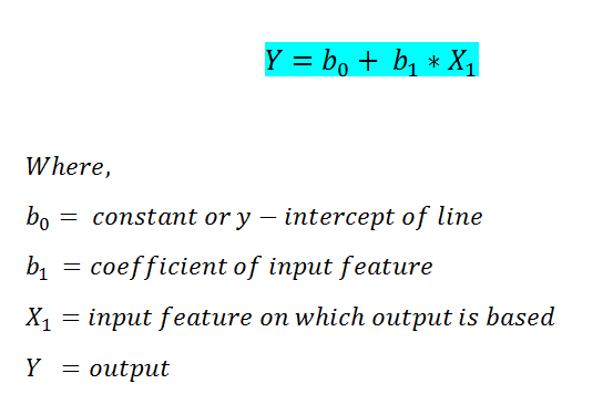
Below we are going to implement simple linear regression using the sklearn library in Python.

Step by step implementation in Python:

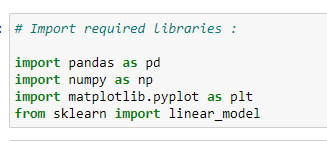
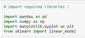
a. Import required libraries:

Since we are going to use various libraries for calculations, we need to import them.

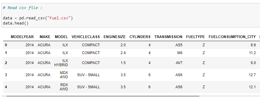
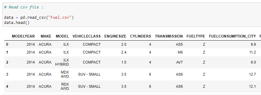
b. Read the CSV file:

We check the first five rows of our dataset. In this case, we are using a vehicle model dataset — please check out the dataset on Softlayer IBM.

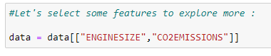
c. Select the features we want to consider in predicting values:

Here our goal is to predict the value of “co2 emissions” from the value of “engine size” in our dataset.

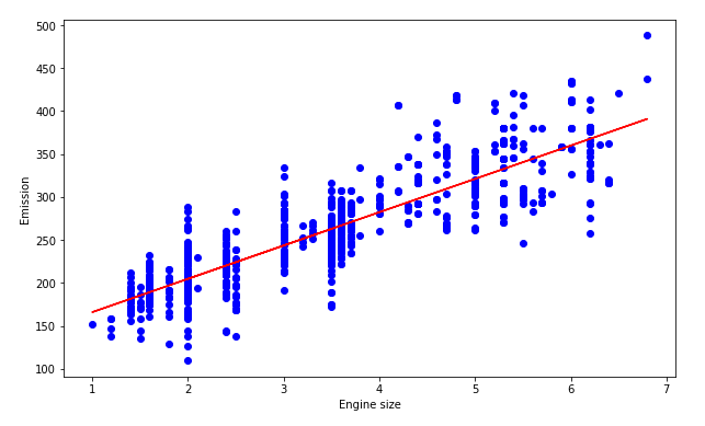
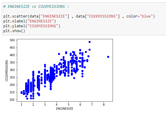
d. Plot the data:

We can visualize our data on a scatter plot.

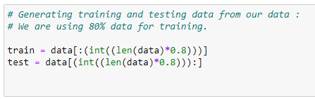
e. Divide the data into training and testing data:

To check the accuracy of a model, we are going to divide our data into training and testing datasets. We will use training data to train our model, and then we will check the accuracy of our model using the testing dataset.

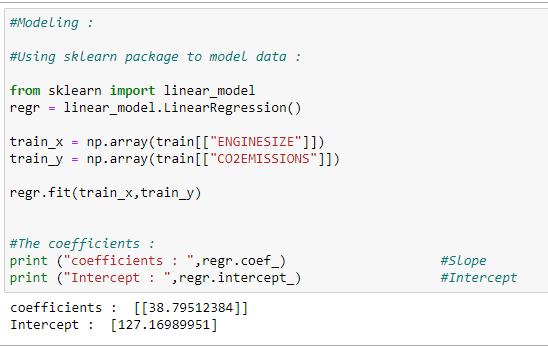
f. Training our model:

Here is how we can train our model and find the coefficients for our best-fit regression line.

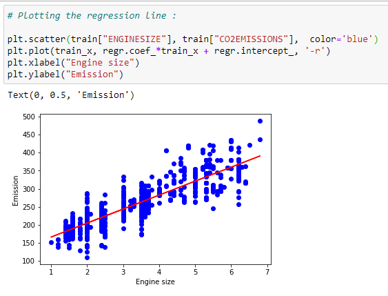
g. Plot the best fit line:

Based on the coefficients, we can plot the best fit line for our dataset.

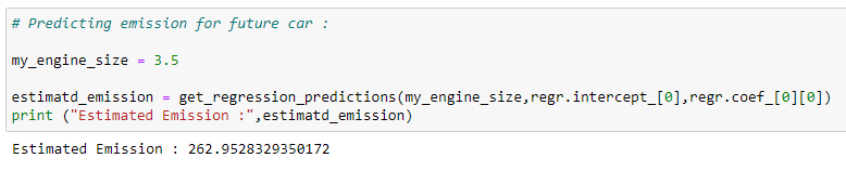
h. Prediction function:

We are going to use a prediction function for our testing dataset.

i. Predicting co2 emissions:

Predicting the values of co2 emissions based on the regression line.

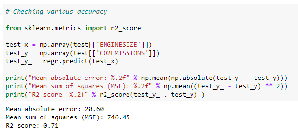
j. Checking accuracy for test data :

We can check the accuracy of a model by comparing the actual values with the predicted values in our dataset.

Putting it all together:

# Import required libraries:
import pandas as pd
import numpy as np
import matplotlib.pyplot as plt
from sklearn import linear_model# Read the CSV file :
data = pd.read_csv(“Fuel.csv”)
data.head()# Let’s select some features to explore more :
data = data[[“ENGINESIZE”,”CO2EMISSIONS”]]# ENGINESIZE vs CO2EMISSIONS:
plt.scatter(data[“ENGINESIZE”] , data[“CO2EMISSIONS”] , color=”blue”)
plt.xlabel(“ENGINESIZE”)
plt.ylabel(“CO2EMISSIONS”)
plt.show()# Generating training and testing data from our data:
# We are using 80% data for training.
train = data[:(int((len(data)*0.8)))]
test = data[(int((len(data)*0.8))):]# Modeling:
# Using sklearn package to model data :
regr = linear_model.LinearRegression()
train_x = np.array(train[[“ENGINESIZE”]])
train_y = np.array(train[[“CO2EMISSIONS”]])
regr.fit(train_x,train_y)# The coefficients:
print (“coefficients : “,regr.coef_) #Slope
print (“Intercept : “,regr.intercept_) #Intercept# Plotting the regression line:
plt.scatter(train[“ENGINESIZE”], train[“CO2EMISSIONS”], color=’blue’)
plt.plot(train_x, regr.coef_*train_x + regr.intercept_, ‘-r’)
plt.xlabel(“Engine size”)
plt.ylabel(“Emission”)# Predicting values:
# Function for predicting future values :
def get_regression_predictions(input_features,intercept,slope):
 predicted_values = input_features*slope + intercept
 return predicted_values# Predicting emission for future car:
my_engine_size = 3.5
estimatd_emission = get_regression_predictions(my_engine_size,regr.intercept_[0],regr.coef_[0][0])
print (“Estimated Emission :”,estimatd_emission)# Checking various accuracy:
from sklearn.metrics import r2_score
test_x = np.array(test[[‘ENGINESIZE’]])
test_y = np.array(test[[‘CO2EMISSIONS’]])
test_y_ = regr.predict(test_x)print(“Mean absolute error: %.2f” % np.mean(np.absolute(test_y_ — test_y)))
print(“Mean sum of squares (MSE): %.2f” % np.mean((test_y_ — test_y) ** 2))
print(“R2-score: %.2f” % r2_score(test_y_ , test_y) )

1.2 Multivariable Linear Regression:

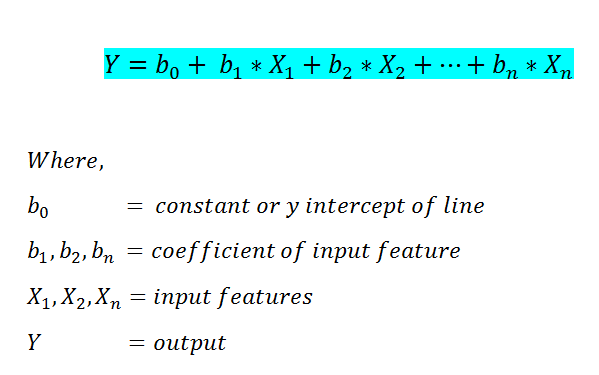
In simple linear regression, we were only able to consider one input feature for predicting the value of the output feature. However, in Multivariable Linear Regression, we can predict the output based on more than one input feature. Here is the formula for multivariable linear regression.

Step by step implementation in Python:

a. Import the required libraries:

b. Read the CSV file :

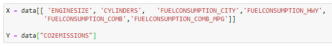
c. Define X and Y:

X stores the input features we want to consider, and Y stores the value of output.

d. Divide data into a testing and training dataset:

Here we are going to use 80% data in training and 20% data in testing.

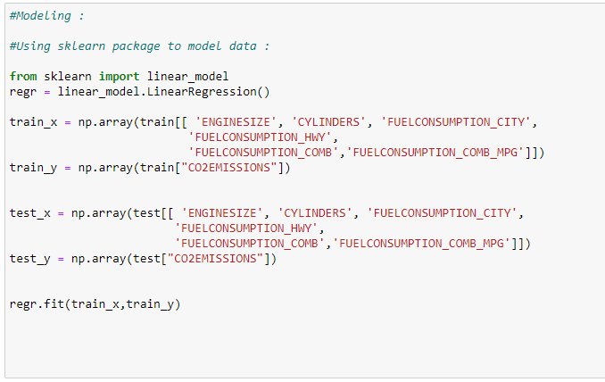
e. Train our model :

Here we are going to train our model with 80% of the data.

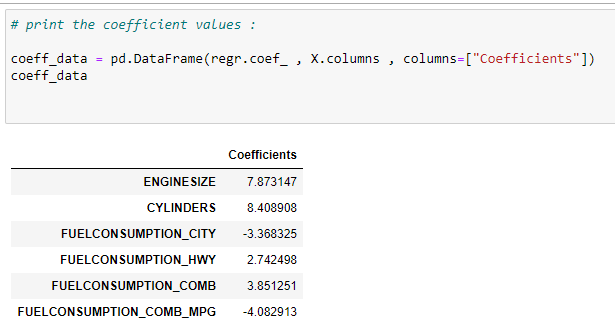
f. Find the coefficients of input features :

Now we need to know which feature has a more significant effect on the output variable. For that, we are going to print the coefficient values. Note that the negative coefficient means it has an inverse effect on the output. i.e., if the value of that features increases, then the output value decreases.

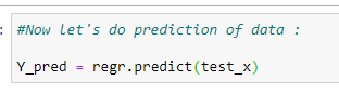
g. Predict the values:

h. Accuracy of the model:

Now notice that here we used the same dataset for simple and multivariable linear regression. We can notice that the accuracy of multivariable linear regression is far better than the accuracy of simple linear regression.

Putting it all together:

# Import the required libraries:
import pandas as pd
import numpy as np
import matplotlib.pyplot as plt
from sklearn import linear_model# Read the CSV file:
data = pd.read_csv(“Fuel.csv”)
data.head()# Consider features we want to work on:
X = data[[ ‘ENGINESIZE’, ‘CYLINDERS’, ‘FUELCONSUMPTION_CITY’,’FUELCONSUMPTION_HWY’, 
 ‘FUELCONSUMPTION_COMB’,’FUELCONSUMPTION_COMB_MPG’]]Y = data[“CO2EMISSIONS”]# Generating training and testing data from our data:
# We are using 80% data for training.
train = data[:(int((len(data)*0.8)))]
test = data[(int((len(data)*0.8))):]#Modeling:
#Using sklearn package to model data :
regr = linear_model.LinearRegression()train_x = np.array(train[[ ‘ENGINESIZE’, ‘CYLINDERS’, ‘FUELCONSUMPTION_CITY’,
 ‘FUELCONSUMPTION_HWY’, ‘FUELCONSUMPTION_COMB’,’FUELCONSUMPTION_COMB_MPG’]])
train_y = np.array(train[“CO2EMISSIONS”])regr.fit(train_x,train_y)test_x = np.array(test[[ ‘ENGINESIZE’, ‘CYLINDERS’, ‘FUELCONSUMPTION_CITY’,
 ‘FUELCONSUMPTION_HWY’, ‘FUELCONSUMPTION_COMB’,’FUELCONSUMPTION_COMB_MPG’]])
test_y = np.array(test[“CO2EMISSIONS”])# print the coefficient values:
coeff_data = pd.DataFrame(regr.coef_ , X.columns , columns=[“Coefficients”])
coeff_data#Now let’s do prediction of data:
Y_pred = regr.predict(test_x)# Check accuracy:
from sklearn.metrics import r2_score
R = r2_score(test_y , Y_pred)
print (“R² :”,R)

1.3 Polynomial Regression:

Sometimes we have data that does not merely follow a linear trend. We sometimes have data that follows a polynomial trend. Therefore, we are going to use polynomial regression.

Before digging into its implementation, we need to know how the graphs of some primary polynomial data look.

Polynomial Functions and Their Graphs:

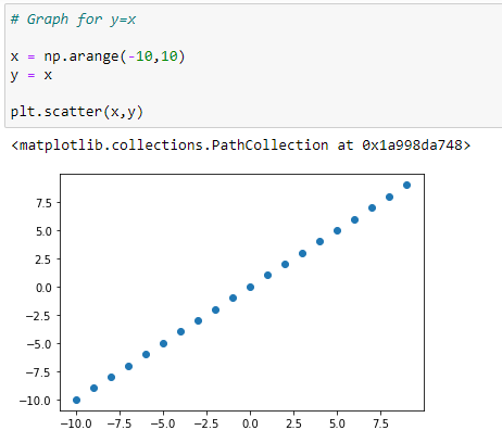
a. Graph for Y=X:

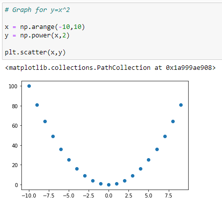
b. Graph for Y = X²:

c. Graph for Y = X³:

d. Graph with more than one polynomials: Y = X³+X²+X:

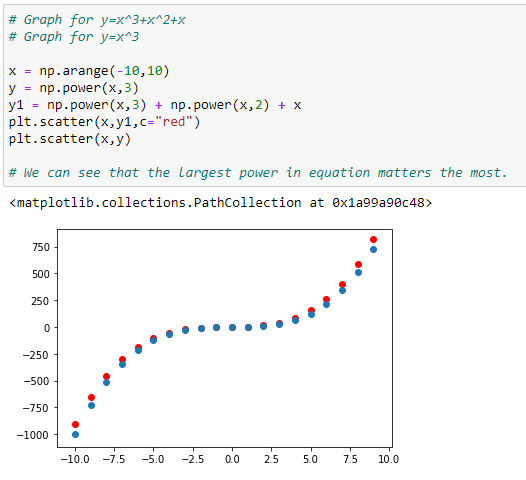
In the graph above, we can see that the red dots show the graph for Y=X³+X²+X and the blue dots shows the graph for Y = X³. Here we can see that the most prominent power influences the shape of our graph.

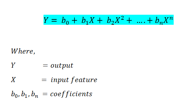
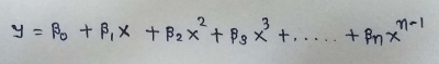
Below is the formula for polynomial regression:

Now in the previous regression models, we used sci-kit learn library for implementation. Now in this, we are going to use Normal Equation to implement it. Here notice that we can use scikit-learn for implementing polynomial regression also, but another method will give us an insight into how it works.

The equation goes as follows:

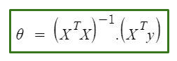
In the equation above:

θ: hypothesis parameters that define it the best.

X: input feature value of each instance.

Y: Output value of each instance.

1.3.1 Hypothesis Function for Polynomial Regression

The main matrix in the standard equation:

Step by step implementation in Python:

a. Import the required libraries:

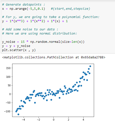
b. Generate the data points:

We are going to generate a dataset for implementing our polynomial regression.

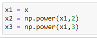
c. Initialize x,x²,x³ vectors:

We are taking the maximum power of x as 3. So our X matrix will have X, X², X³.

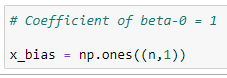
d. Column-1 of X matrix:

The 1st column of the main matrix X will always be 1 because it holds the coefficient of beta_0.

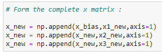
e. Form the complete x matrix:

Look at the matrix X at the start of this implementation. We are going to create it by appending vectors.

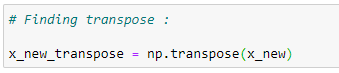
f. Transpose of the matrix:

We are going to calculate the value of theta step-by-step. First, we need to find the transpose of the matrix.

g. Matrix multiplication:

After finding the transpose, we need to multiply it with the original matrix. Keep in mind that we are going to implement it with a normal equation, so we have to follow its rules.

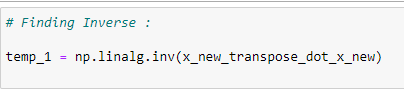
h. The inverse of a matrix:

Finding the inverse of the matrix and storing it in temp1.

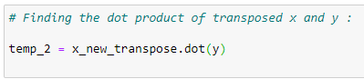
i. Matrix multiplication:

Finding the multiplication of transposed X and the Y vector and storing it in the temp2 variable.

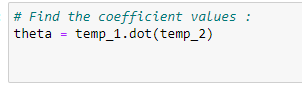
j. Coefficient values:

To find the coefficient values, we need to multiply temp1 and temp2. See the Normal Equation formula.

k. Store the coefficients in variables:

Storing those coefficient values in different variables.

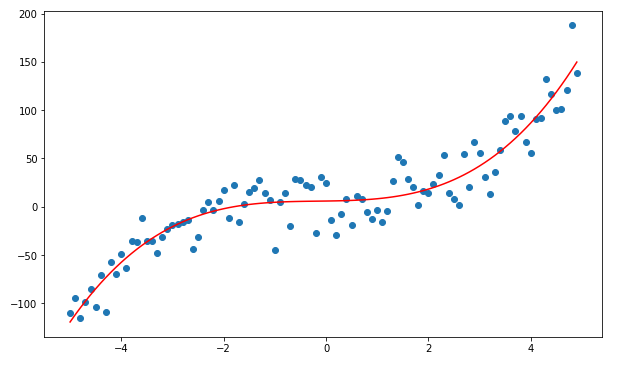
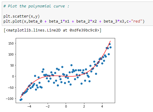
l. Plot the data with curve:

Plotting the data with the regression curve.

m. Prediction function:

Now we are going to predict the output using the regression curve.

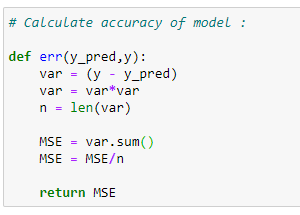
n. Error function:

Calculate the error using mean squared error function.

o. Calculate the error:

Putting it all together:

# Import required libraries:
import numpy as np
import matplotlib.pyplot as plt# Generate datapoints:
x = np.arange(-5,5,0.1)
y_noise = 20 * np.random.normal(size = len(x))
y = 1*(x**3) + 1*(x**2) + 1*x + 3+y_noise
plt.scatter(x,y)# Make polynomial data:
x1 = x
x2 = np.power(x1,2)
x3 = np.power(x1,3)# Reshaping data:
x1_new = np.reshape(x1,(n,1))
x2_new = np.reshape(x2,(n,1))
x3_new = np.reshape(x3,(n,1))# First column of matrix X:
x_bias = np.ones((n,1))# Form the complete x matrix:
x_new = np.append(x_bias,x1_new,axis=1)
x_new = np.append(x_new,x2_new,axis=1)
x_new = np.append(x_new,x3_new,axis=1)# Finding transpose:
x_new_transpose = np.transpose(x_new)# Finding dot product of original and transposed matrix :
x_new_transpose_dot_x_new = x_new_transpose.dot(x_new)# Finding Inverse:
temp_1 = np.linalg.inv(x_new_transpose_dot_x_new)# Finding the dot product of transposed x and y :
temp_2 = x_new_transpose.dot(y)# Finding coefficients:
theta = temp_1.dot(temp_2)
theta# Store coefficient values in different variables:
beta_0 = theta[0]
beta_1 = theta[1]
beta_2 = theta[2]
beta_3 = theta[3]# Plot the polynomial curve:
plt.scatter(x,y)
plt.plot(x,beta_0 + beta_1*x1 + beta_2*x2 + beta_3*x3,c=”red”)# Prediction function:
def prediction(x1,x2,x3,beta_0,beta_1,beta_2,beta_3):
 y_pred = beta_0 + beta_1*x1 + beta_2*x2 + beta_3*x3
 return y_pred
 
# Making predictions:
pred = prediction(x1,x2,x3,beta_0,beta_1,beta_2,beta_3)
 
# Calculate accuracy of model:
def err(y_pred,y):
 var = (y — y_pred)
 var = var*var
 n = len(var)
 MSE = var.sum()
 MSE = MSE/n
 
 return MSE# Calculating the error:
error = err(pred,y)
error

1.4 Exponential Regression:

Some real-life examples of exponential growth:

1. Microorganisms in cultures.

2. Spoilage of food.

3. Human Population.

4. Compound Interest.

5. Pandemics (Such as Covid-19).

6. Ebola Epidemic.

7. Invasive Species.

8. Fire.

9. Cancer Cells.

10. Smartphone Uptake and Sale.

The formula for exponential regression is as follow:

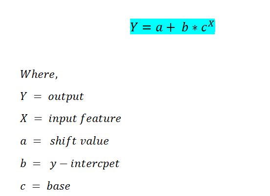
In this case, we are going to use the scikit-learn library to find the coefficient values such as a, b, c.

Step by step implementation in Python

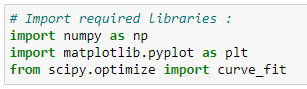
a. Import the required libraries:

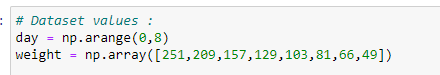
b. Insert the data points:

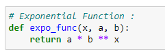
c. Implement the exponential function algorithm:

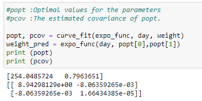
d. Apply optimal parameters and covariance:

Here we use curve_fit to find the optimal parameter values. It returns two variables, called popt, pcov.

popt stores the value of optimal parameters, and pcov stores the values of its covariances. We can see that popt variable has two values. Those values are our optimal parameters. We are going to use those parameters and plot our best fit curve, as shown below.

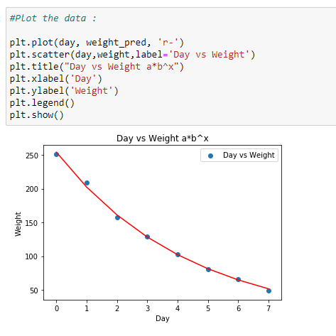
e. Plot the data:

Plotting the data with the coefficients found.

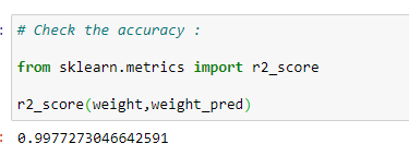
f. Check the accuracy of the model:

Check the accuracy of the model with r2_score.

Putting it all together:

# Import required libraries:
import numpy as np
import matplotlib.pyplot as plt
from scipy.optimize import curve_fit# Dataset values :
day = np.arange(0,8)
weight = np.array([251,209,157,129,103,81,66,49])# Exponential Function :
def expo_func(x, a, b):
 return a * b ** x#popt :Optimal values for the parameters
#pcov :The estimated covariance of poptpopt, pcov = curve_fit(expo_func, day, weight)
weight_pred = expo_func(day,popt[0],popt[1])# Plotting the data
plt.plot(day, weight_pred, ‘r-’)
plt.scatter(day,weight,label=’Day vs Weight’)
plt.title(“Day vs Weight a*b^x”)
plt.xlabel(‘Day’)
plt.ylabel(‘Weight’)
plt.legend()
plt.show()# Equation
a=popt[0].round(4)
b=popt[1].round(4)
print(f’The equation of regression line is y={a}*{b}^x’

Exponential Regression — https://towardsai.net/machine-learning-algorithms

1.5 Sinusoidal Regression:

Some real-life examples of sinusoidal regression:

1. Generation of music waves.
2. Sound travels in waves.
3. Trigonometric functions in constructions.
4. Used in space flights.
5. GPS location calculations.
6. Architecture.
7. Electrical current.
8. Radio broadcasting.
9. Low and high tides of the ocean.
10. Buildings.

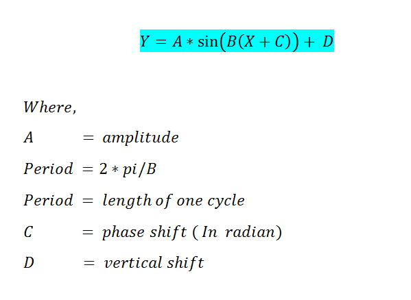
Sometimes we have data that shows patterns like a sine wave. Therefore, in such case scenarios, we use a sinusoidal regression. Below we can show the formula for the algorithm:

Step by step implementation in Python:

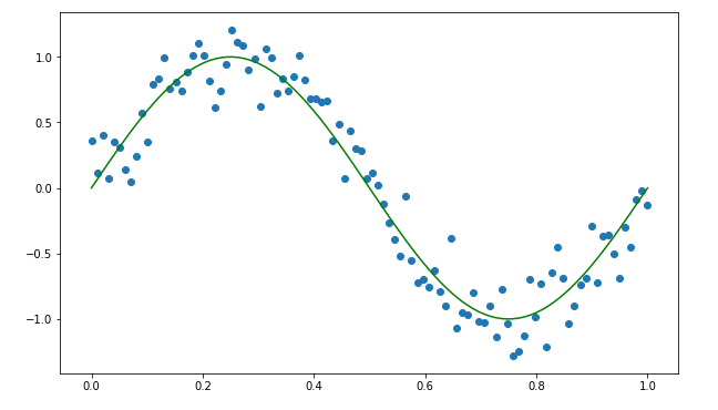
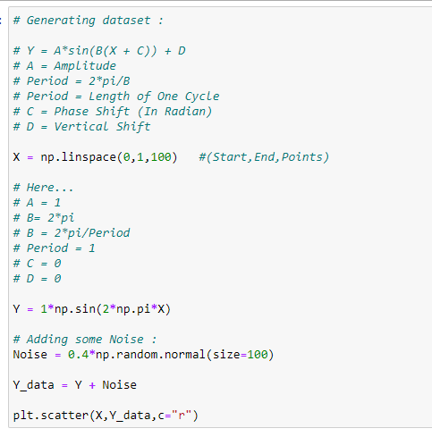
a. Generating the dataset:

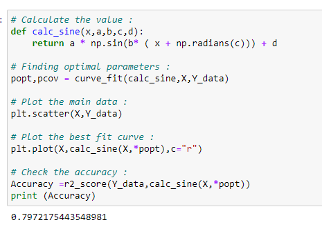
b. Applying a sine function:

Here we have created a function called “calc_sine” to calculate the value of output based on optimal coefficients. Here we will use the scikit-learn library to find the optimal parameters.

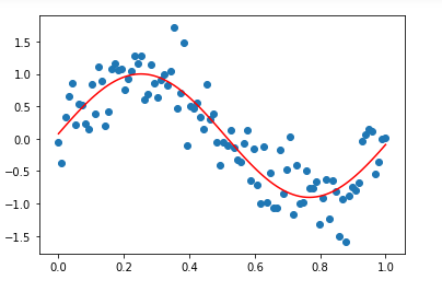
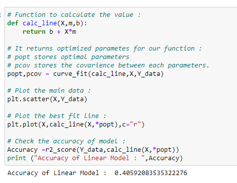
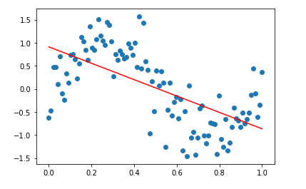
c. Why does a sinusoidal regression perform better than linear regression?

If we check the accuracy of the model after fitting our data with a straight line, we can see that the accuracy in prediction is less than that of sine wave regression. That is why we use sinusoidal regression.

Putting it all together:

# Import required libraries:
import numpy as np
import matplotlib.pyplot as plt
from scipy.optimize import curve_fit
from sklearn.metrics import r2_score# Generating dataset:# Y = A*sin(B(X + C)) + D
# A = Amplitude
# Period = 2*pi/B
# Period = Length of One Cycle
# C = Phase Shift (In Radian)
# D = Vertical ShiftX = np.linspace(0,1,100) #(Start,End,Points)# Here…
# A = 1
# B= 2*pi
# B = 2*pi/Period
# Period = 1
# C = 0
# D = 0Y = 1*np.sin(2*np.pi*X)# Adding some Noise :
Noise = 0.4*np.random.normal(size=100)Y_data = Y + Noiseplt.scatter(X,Y_data,c=”r”)# Calculate the value:
def calc_sine(x,a,b,c,d):
 return a * np.sin(b* ( x + np.radians(c))) + d# Finding optimal parameters :
popt,pcov = curve_fit(calc_sine,X,Y_data)# Plot the main data :
plt.scatter(X,Y_data)# Plot the best fit curve :
plt.plot(X,calc_sine(X,*popt),c=”r”)# Check the accuracy :
Accuracy =r2_score(Y_data,calc_sine(X,*popt))
print (Accuracy)# Function to calculate the value :
def calc_line(X,m,b):
 return b + X*m# It returns optimized parametes for our function :
# popt stores optimal parameters
# pcov stores the covarience between each parameters.
popt,pcov = curve_fit(calc_line,X,Y_data)# Plot the main data :
plt.scatter(X,Y_data)# Plot the best fit line :
plt.plot(X,calc_line(X,*popt),c=”r”)# Check the accuracy of model :
Accuracy =r2_score(Y_data,calc_line(X,*popt))
print (“Accuracy of Linear Model : “,Accuracy)

Sinusoidal Regression — https://towardsai.net/machine-learning-algorithms

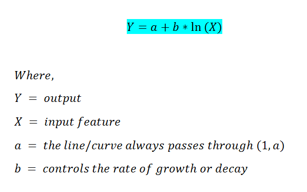
1.6 Logarithmic Regression:

Some real-life examples of logarithmic growth:

1. The magnitude of earthquakes.
2. The intensity of sound.
3. The acidity of a solution.
4. The pH level of solutions.
5. Yields of chemical reactions.
6. Production of goods.
7. Growth of infants.
8. A COVID-19 graph.

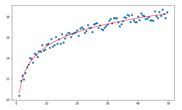
Sometimes we have data that grows exponentially in the statement, but after a certain point, it goes flat. In such a case, we can use a logarithmic regression.

Step by step implementation in Python:

a. Import required libraries:

b. Generating the dataset:

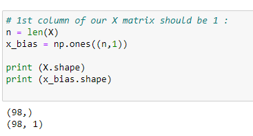
c. The first column of our matrix X :

Here we will use our normal equation to find the coefficient values.

d. Reshaping X:

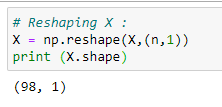
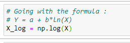
e. Going with the Normal Equation formula:

f. Forming the main matrix X:

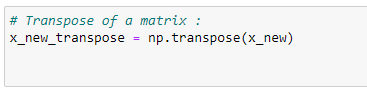
g. Finding the transpose matrix:

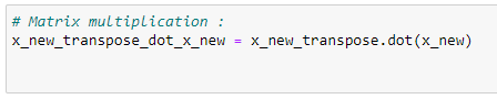
h. Performing matrix multiplication:

i. Finding the inverse:

j. Matrix multiplication:

k. Finding the coefficient values:

l. Plot the data with the regression curve:

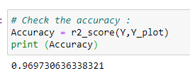
m. Accuracy:

Putting it all together:

# Import required libraries:
import numpy as np
import matplotlib.pyplot as plt
from sklearn.metrics import r2_score# Dataset:
# Y = a + b*ln(X)
X = np.arange(1,50,0.5)
Y = 10 + 2*np.log(X)#Adding some noise to calculate error!
Y_noise = np.random.rand(len(Y))
Y = Y +Y_noise
plt.scatter(X,Y)# 1st column of our X matrix should be 1:
n = len(X)
x_bias = np.ones((n,1))print (X.shape)
print (x_bias.shape)# Reshaping X :
X = np.reshape(X,(n,1))
print (X.shape)# Going with the formula:
# Y = a + b*ln(X)
X_log = np.log(X)# Append the X_log to X_bias:
x_new = np.append(x_bias,X_log,axis=1)# Transpose of a matrix:
x_new_transpose = np.transpose(x_new)# Matrix multiplication:
x_new_transpose_dot_x_new = x_new_transpose.dot(x_new)# Find inverse:
temp_1 = np.linalg.inv(x_new_transpose_dot_x_new)# Matrix Multiplication:
temp_2 = x_new_transpose.dot(Y)# Find the coefficient values:
theta = temp_1.dot(temp_2)# Plot the data:
a = theta[0]
b = theta[1]
Y_plot = a + b*np.log(X)
plt.scatter(X,Y)
plt.plot(X,Y_plot,c=”r”)# Check the accuracy:
Accuracy = r2_score(Y,Y_plot)
print (Accuracy)

Logarithmic Regression — https://towardsai.net/machine-learning-algorithms

DISCLAIMER: The views expressed in this article are those of the author(s) and do not represent the views of Carnegie Mellon University, nor other companies (directly or indirectly) associated with the author(s). These writings do not intend to be final products, yet rather a reflection of current thinking, along with being a catalyst for discussion and improvement.

Citation

For attribution in academic contexts, please cite this work as:

Shukla, et al., “Machine Learning Algorithms For Beginners with Code Examples in Python”, Towards AI, 2020

BibTex citation:

@article{pratik_iriondo_chen_2020, 
 title={Machine Learning Algorithms For Beginners with Code Examples in Python}, 
 url={https://towardsai.net/machine-learning-algorithms}, 
 journal={Towards AI}, 
 publisher={Towards AI Co.}, 
 author={Pratik, Shukla and Iriondo, 
 Roberto and Chen, Sherwin}, 
 editor={Stanford, StacyEditor}, 
 year={2020}, 
 month={Jun}
}