Imagine asking a computer to identify a picture of a cat or a dog without any supporting data; the computer has a 50/50 chance of being correct in this scenario. Now, imagine writing a program that teaches a computer how to actively learn the difference between the animals by analyzing photos of both.
This is the essence of machine learning. As humans, we learn from experience while machines generally follow our instructions. However, with machine learning, we can train computers to learn from data and perform high-level analyses and predictions. Machine learning is one of modern technology’s most promising concepts, one with boundless applications across most industries.
If you’re interested in a technology-related career, there’s a good chance that a working knowledge of machine learning will make you more marketable. In fact, some jobs focus specifically on incorporating machine learning advancements in order to help businesses gain a competitive advantage
What Is Machine Learning?
The simplest machine learning definition is this: the science of teaching computers how to learn like humans. Machine learning requires algorithms to examine huge datasets, find patterns within that data, and then make assessments and predictions based on those patterns. Essentially, it is a branch of artificial intelligence (AI) that shifts the rules of programming as we conventionally understand them.
Normally, programmers write programs where they input data and rules and the computer follows those rules to produce an answer. With machine learning, programmers input the data and the answer, and the computer determines the rules for producing that answer. In the earlier pet picture example, programmers would input the answer (“This is a photo of a cat”), the data (photos of cats and dogs), and the computer would use an algorithm to learn the difference.
Machine learning is applied in many familiar ways. Your favorite streaming service uses machine learning to recommend movies and shows based on your viewing habits; financial institutions use it to spot fraud in billions of transactions and devise ways to prevent it; self-driving cars use it to learn directional commands; and phones use it to enact accurate facial recognition.
According to a 2020 study, the global size of the machine learning market was valued at $6.9 billion in 2018. It is projected to increase nearly 44 percent through 2025 as companies seek to optimize their supply chains and use more digital resources to reach customers.
To be effective, machine learning needs detailed pieces of data from diverse sources. Algorithms learn best when they can apply vast amounts of data to a specific model. For example, the more photos of dogs and cats you input, the better the algorithm will become in identifying the differences between the animals.
The term “machine learning” is often used synonymously with artificial intelligence and, while these concepts share similarities, they are generally used for different purposes. AI is the broad science of training machines to perform human tasks, while machine learning is one of many AI-based methods of accomplishing that training.
Machine Learning Algorithm Types
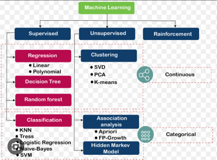
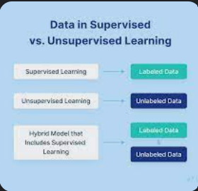
Algorithms are the procedures that computers use to perform pattern recognition on data models and create an output. Many types of algorithms exist, and they fall into four primary groups: supervised learning, unsupervised learning, semi-supervised learning, and reinforcement learning.
Supervised Learning
Supervised learning is a process where labeled input data and the correct answers are both given to a computer so that it can learn how to reach the correct answer on its own. The correct answer, or output, can refer to an object, a situation, or a problem that needs to be solved.
There are two types of supervised learning: classification and regression. Classification is simply the process of sorting identified data into groups. To illustrate, let’s apply classification to our cats and dogs example: The programmer inputs labeled photos of cats and dogs so the computer knows which photo shows which type of animal. Using that training data set to learn how to identify the pictures, the computer can then apply its knowledge to a new data set and label them correctly. The more photos the computer analyzes, the faster and more accurate it becomes at classifying the data.
The second type of supervised learning is regression, which enables the computer to forecast likely future or desirable outcomes from a labeled data set. Different types of regression are used to forecast future sales, anticipated stock performanced, or the impact of financial events on the global economy. However, regression can be used for far more than financial analysis.
Here are some other examples:
Social Media
Facebook offers you a friend suggestion because it recognizes your friend in a photo album of tagged pictures.
Streaming Suggestions
Netflix recommends movies for you to watch based on your past viewing choices, ratings, and the viewing habits of subscribers with similar tastes.
Predicting Home Prices
Realtors use machine learning to analyze housing data (location, square footage, number of bedrooms, added features like pools, etc.) in comparison to other properties to understand not only how to best price a property, but also how that price will impact days on the market and likely closing dates for their clients.
Suggesting Further Purchases
When you check out a cart full of items at the grocery store, those purchases become data. Retailers use that data in many ways — such as predicting future purchases, making suggestions, or offering coupons as incentives.
Unsupervised Learning
Unsupervised learning refers to the process in which a computer finds nonintuitive patterns in unlabeled data. It’s different from supervised learning because the datasets are not labeled and the computer is not given a specific question to answer.
There are many different types of unsupervised learning including K-means clustering, hierarchical clustering, anomaly detection, and principal component analysis to name a few. The most commonly discussed uses are clustering and anomaly detection.
Clustering is used to find natural groups, or clusters, within a dataset. These clusters can be analyzed to group like customers together (e.g, customer segmentation), identify products that are purchased at the same time (e.g., peanut butter and jelly), or better understand the attributes of successful executives (e.g., technical skills, personality profile, education).
In our dogs and cats example, assume you input pictures of dogs and cats but don’t label them. Using clustering, the computer will look for common traits (body types, floppy ears, whiskers, etc.) and group the photos. However, while you may expect the computer to group the photos by dogs vs. cats, it could group them by fur color, coat length, or size. The benefit of clustering is that the computer will find nonintuitive ways of looking at data which enable the discovery of new data trends (e.g., there are twice as many long-coated animals as short-coated) which allow for new marketing opportunities (e.g., dry pet shampoo and brush marketing increases).
In anomaly detection, however, the computer looks for rare differences rather than commonalities. For example, if we used anomaly detection on our dog and cat photos, the computer might flag the photo of a Sphynx cat because it is hairless or an albino dog due to its lack of color.
Here are some other applications of anomaly detection.
Finding Fraud
Banks analyze all sorts of transactions: deposits, withdrawals, loan repayments, etc. Unsupervised learning can group these data points and flag outlier transactions (e.g., transactions that don’t align with the majority of data points) that may indicate fraud.
Consumer Studies
Companies use anomaly detection to identify and understand actions competitors may take in the marketplace. For example, a retailer may expect to take three share points in every new market they open a store during the first month of operations; however, they may notice certain new stores are underperforming and don’t know why. Anomaly detection can be used to identify likely competitive activity which is preventing share growth. Specifically, the anomaly of common products not being found in their shoppers’ baskets (e.g., bread, milk, eggs, chicken breast) which may indicate covert competitor incentives that are successfully impacting the retailer’s shopper frequency and average order size.
Image Recognition
Computers use unsupervised learning to perform all sorts of image recognition tasks including facial recognition to open your mobile phone and healthcare imaging where identifying cell-structure anomalies can assist in cancer diagnosis and treatment.
Semi-Supervised Learning
Semi-supervised learning is essentially a combination of supervised and unsupervised learning techniques. It merges a small amount of manually labeled data (a supervised learning element) as a basis for autonomously defining a large amount of unlabeled data (an unsupervised element). Through data clustering, this method makes it possible to train a machine learning algorithm (ML algorithm) on data annotation (e.g., the labeling or classification of data) without manually labeling all of the training data first, potentially increasing efficiency without sacrificing quality or accuracy.
For example, if you have a large data set consisting of dogs and cats, a semi-supervised approach would allow you to manually label a small portion of that data (identifying a few pictures as “dogs” and a few others as “cats”), and the ML algorithm would then be equipped to properly define the remaining data. This blends the benefits of supervised and unsupervised learning by nudging the algorithm to make strong autonomous decisions with less initial human oversight.
Image Classification
While higher-level image classification often requires a fully supervised approach (due to the necessary labeling of a large amount of initial training data), specific image classification scenarios can benefit from semi-supervised learning. For example, to annotate images of handwritten numbers, training data must be clustered to include the most representative variations of the written numbers and can then be used to inform the ML algorithm. In turn, the algorithm should be able to identify unlabeled images of handwritten numbers with relatively high accuracy, yielding the intended outcome with less initial oversight.
Document Classification
Similarly, semi-supervised learning can be useful in document classification, eliminating the need for human workers to read through numerous text documents just to broadly classify them. A semi-supervised approach allows the algorithm to learn from a relatively small amount of text data so that it can identify and classify the larger amount of unlabeled documents.
Reinforcement Learning
Reinforcement learning is the process by which a computer learns how to behave in a certain environment by performing an action and seeing a specific result. In this process, the key terms to know are agents and environments. Agents interact with the environment through actions and receive feedback regarding those actions. Consider it similar to the first time you (the agent) touched a hot stove (the environment) — the feedback from the action (e.g., pain of touching the stove) reinforced the idea that you shouldn’t touch a hot stove again.
Reinforcement can also be applied to our cats and dogs scenario. If you input an image of a dog and the computer says it’s a cat, you can then correct that answer. The computer will learn from that correction, or reinforcement, and increase its ability to properly identify the image over time and through repetition of the process.
Reinforcement is a growing method of machine learning because of its applications in robotics and automation. Consider these examples:
Self-Driving Cars
Autonomous vehicles interpret a huge amount of data through cameras, sensors, and radar that monitor their surroundings. Reinforcement learning contributes to the real-time decision-making process.
Industry Automation
Companies automate tasks in warehouses and production facilities through robotics that operate on reinforcement learning models.
Healthcare
Reinforcement learning is becoming more common in medicine because its methodology (e.g., learning from interactions in an environment) often mirrors that of diagnosis and treating diseases.
Gaming
Reinforcement learning algorithms are popular for video games because they learn quickly and can mimic human performance. Reinforcement is one way computers learn how to master games from chess to complex video games, allowing bot players to engage with human players in a realistic way.
Machine Learning Jobs
As we look to automate more processes at work and in our daily lives, machine learning will become more valuable. Machine learning is important to data science, artificial intelligence, and robotics (among many other fields).
Where can knowledge of machine learning take you? Here are a few potential careers to consider.
Machine Learning Engineer: Though coding is required, this role is a bit different than that of a computer programmer. Machine learning engineers build programs that teach computers how to identify patterns and perform tasks based on those patterns. This is an ideal career path for those who want to get into robotics.
Machine Learning Data Scientist: Data scientists combine statistics, programming, and data analysis to generate insight from data — a skill that is in high demand. According to the U.S. Bureau of Labor Statistics (BLS), the demand for computer and information research scientists is expected to grow by 15 percent through 2029. Machine learning is an important component of becoming a data scientist.
NLP Scientist: When you ask Siri or Alexa a question, they answer because of natural language processing (NLP). NLP scientists work in a unique world of textual data analysis, linguistics, and computer programming to facilitate communication between humans and machines.
Business Intelligence Developer: Companies need ways to harness, assess, and report all the data they collect, and business intelligence (BI) provides that framework. BI developers work with data warehouses, visualization software, and other tools to explain what is happening. BI is also vital in generating ways to benefit from consumer data.
Data Analyst: Want to help companies and organizations make sense of their data? Then you may want to consider becoming a data analyst. You’ll learn how to mix statistics, business knowledge, and communication skills to bring data to life. As data generation grows, so do the job prospects for analysts. The BLS projects a 25 percent increase by 2029.
Want to learn more about the function of machine learning in data science? Check out this guide to understanding data science roles.
Machine Learning FAQs
What is machine learning like for beginners?
Machine learning requires a solid foundation in fields like math, statistics, and programming. Calculus and linear algebra are important starting points, as is the ability to code. A great way to learn about machine learning, and other data science skills, is to enroll in a data science boot camp.
What is a good introduction to machine learning?
What is an example of machine learning?
Ready to take the next step in a career that involves machine learning? Consider a bootcamp in data science and analytics. The 24-week online program at Georgia Tech Data Science and Analytics Boot Camp is a great way to learn in-demand skills to get you ready for your job search. Contact us today to get started.
Machine learning (ML) is rapidly changing the world, from diverse types of applications and research pursued in industry and academia. Machine learning is affecting every part of our daily lives. From voice assistants using NLP and machine learning to make appointments, check our calendar, and play music, to programmatic advertisements — that are so accurate that they can predict what we will need before we even think of it.
More often than not, the complexity of the scientific field of machine learning can be overwhelming, making keeping up with “what is important” a very challenging task. However, to make sure that we provide a learning path to those who seek to learn machine learning, but are new to these concepts. In this article, we look at the most critical basic algorithms that hopefully make your machine learning journey less challenging.
Any suggestions or feedback is crucial to continue to improve. Please let us know in the comments if you have any.
Index
Introduction to Machine Learning.
Major Machine Learning Algorithms.
Supervised vs. Unsupervised Learning.
Linear Regression.
Multivariable Linear Regression.
Polynomial Regression.
Exponential Regression.
Sinusoidal Regression.
Logarithmic Regression.
What is machine learning?
A computer program is said to learn from experience E with respect to some class of tasks T and performance measure P, if its performance at tasks in T, as measured by P, improves with experience E. ~ Tom M. Mitchell [1]
Machine learning behaves similarly to the growth of a child. As a child grows, her experience E in performing task T increases, which results in higher performance measure (P).
For instance, we give a “shape sorting block” toy to a child. (Now we all know that in this toy, we have different shapes and shape holes). In this case, our task T is to find an appropriate shape hole for a shape. Afterward, the child observes the shape and tries to fit it in a shaped hole. Let us say that this toy has three shapes: a circle, a triangle, and a square. In her first attempt at finding a shaped hole, her performance measure(P) is 1/3, which means that the child found 1 out of 3 correct shape holes.
Second, the child tries it another time and notices that she is a little experienced in this task. Considering the experience gained (E), the child tries this task another time, and when measuring the performance(P), it turns out to be 2/3. After repeating this task (T) 100 times, the baby now figured out which shape goes into which shape hole.
So her experience (E) increased, her performance(P) also increased, and then we notice that as the number of attempts at this toy increases. The performance also increases, which results in higher accuracy.
Such execution is similar to machine learning. What a machine does is, it takes a task (T), executes it, and measures its performance (P). Now a machine has a large number of data, so as it processes that data, its experience (E) increases over time, resulting in a higher performance measure (P). So after going through all the data, our machine learning model’s accuracy increases, which means that the predictions made by our model will be very accurate.
Another definition of machine learning by Arthur Samuel:
Machine Learning is the subfield of computer science that gives “computers the ability to learn without being explicitly programmed.” ~ Arthur Samuel [2]
Let us try to understand this definition: It states “learn without being explicitly programmed” — which means that we are not going to teach the computer with a specific set of rules, but instead, what we are going to do is feed the computer with enough data and give it time to learn from it, by making its own mistakes and improve upon those. For example, We did not teach the child how to fit in the shapes, but by performing the same task several times, the child learned to fit the shapes in the toy by herself.
Therefore, we can say that we did not explicitly teach the child how to fit the shapes. We do the same thing with machines. We give it enough data to work on and feed it with the information we want from it. So it processes the data and predicts the data accurately.
Why do we need machine learning?
For instance, we have a set of images of cats and dogs. What we want to do is classify them into a group of cats and dogs. To do that we need to find out different animal features, such as:
How many eyes does each animal have?
What is the eye color of each animal?
What is the height of each animal?
What is the weight of each animal?
What does each animal generally eat?
We form a vector on each of these questions’ answers. Next, we apply a set of rules such as:
If height > 1 feet and weight > 15 lbs, then it could be a cat.
Now, we have to make such a set of rules for every data point. Furthermore, we place a decision tree of if, else if, else statements and check whether it falls into one of the categories.
Let us assume that the result of this experiment was not fruitful as it misclassified many of the animals, which gives us an excellent opportunity to use machine learning.
What machine learning does is process the data with different kinds of algorithms and tells us which feature is more important to determine whether it is a cat or a dog. So instead of applying many sets of rules, we can simplify it based on two or three features, and as a result, it gives us a higher accuracy. The previous method was not generalized enough to make predictions.
Machine learning models helps us in many tasks, such as:
Object Recognition
Summarization
Prediction
Classification
Clustering
Recommender systems
And others
What is a machine learning model?
A machine learning model is a question/answering system that takes care of processing machine-learning related tasks. Think of it as an algorithm system that represents data when solving problems. The methods we will tackle below are beneficial for industry-related purposes to tackle business problems.
For instance, let us imagine that we are working on Google Adwords’ ML system, and our task is to implementing an ML algorithm to convey a particular demographic or area using data. Such a task aims to go from using data to gather valuable insights to improve business outcomes.
Major Machine Learning Algorithms:
1. Regression (Prediction)
We use regression algorithms for predicting continuous values.
Regression algorithms:
Linear Regression
Polynomial Regression
Exponential Regression
Logistic Regression
Logarithmic Regression
2. Classification
We use classification algorithms for predicting a set of items’ class or category.
Classification algorithms:
K-Nearest Neighbors
Decision Trees
Random Forest
Support Vector Machine
Naive Bayes
3. Clustering
We use clustering algorithms for summarization or to structure data.
Clustering algorithms:
K-means
DBSCAN
Mean Shift
Hierarchical
4. Association
We use association algorithms for associating co-occurring items or events.
Association algorithms:
Apriori
5. Anomaly Detection
We use anomaly detection for discovering abnormal activities and unusual cases like fraud detection.
6. Sequence Pattern Mining
We use sequential pattern mining for predicting the next data events between data examples in a sequence.
7. Dimensionality Reduction
We use dimensionality reduction for reducing the size of data to extract only useful features from a dataset.
8. Recommendation Systems
We use recommenders algorithms to build recommendation engines.
Examples:
Netflix recommendation system.
A book recommendation system.
A product recommendation system on Amazon.
Nowadays, we hear many buzz words like artificial intelligence, machine learning, deep learning, and others.
What are the fundamental differences between Artificial Intelligence, Machine Learning, and Deep Learning?
Artificial Intelligence (AI):
Artificial intelligence (AI), as defined by Professor Andrew Moore, is the science and engineering of making computers behave in ways that, until recently, we thought required human intelligence [4].
These include:
Computer Vision
Language Processing
Creativity
Summarization
Machine Learning (ML):
As defined by Professor Tom Mitchell, machine learning refers to a scientific branch of AI, which focuses on the study of computer algorithms that allow computer programs to automatically improve through experience [3].
These include:
Classification
Neural Network
Clustering
Deep Learning:
Deep learning is a subset of machine learning in which layered neural networks, combined with high computing power and large datasets, can create powerful machine learning models. [3]
Neural network abstract representation | Photo by Clink Adair via Unsplash
Why do we prefer Python to implement machine learning algorithms?
Python is a popular and general-purpose programming language. We can write machine learning algorithms using Python, and it works well. The reason why Python is so popular among data scientists is that Python has a diverse variety of modules and libraries already implemented that make our life more comfortable.
Let us have a brief look at some exciting Python libraries.
Numpy: It is a math library to work with n-dimensional arrays in Python. It enables us to do computations effectively and efficiently.
Scipy: It is a collection of numerical algorithms and domain-specific tool-box, including signal processing, optimization, statistics, and much more. Scipy is a functional library for scientific and high-performance computations.
Matplotlib: It is a trendy plotting package that provides 2D plotting as well as 3D plotting.
Scikit-learn: It is a free machine learning library for python programming language. It has most of the classification, regression, and clustering algorithms, and works with Python numerical libraries such as Numpy, Scipy.
Machine learning algorithms classify into two groups :
Supervised Learning algorithms
Unsupervised Learning algorithms
I. Supervised Learning Algorithms:
Goal: Predict class or value label.
Supervised learning is a branch of machine learning(perhaps it is the mainstream of machine/deep learning for now) related to inferring a function from labeled training data. Training data consists of a set of *(input, target)* pairs, where the input could be a vector of features, and the target instructs what we desire for the function to output. Depending on the type of the *target*, we can roughly divide supervised learning into two categories: classification and regression. Classification involves categorical targets; examples ranging from some simple cases, such as image classification, to some advanced topics, such as machine translations and image caption. Regression involves continuous targets. Its applications include stock prediction, image masking, and others- which all fall in this category.
To illustrate the example of supervised learning below | Source: Photo by Shirota Yuri, Unsplash
To understand what supervised learning is, we will use an example. For instance, we give a child 100 stuffed animals in which there are ten animals of each kind like ten lions, ten monkeys, ten elephants, and others. Next, we teach the kid to recognize the different types of animals based on different characteristics (features) of an animal. Such as if its color is orange, then it might be a lion. If it is a big animal with a trunk, then it may be an elephant.
We teach the kid how to differentiate animals, this can be an example of supervised learning. Now when we give the kid different animals, he should be able to classify them into an appropriate animal group.
For the sake of this example, we notice that 8/10 of his classifications were correct. So we can say that the kid has done a pretty good job. The same applies to computers. We provide them with thousands of data points with its actual labeled values (Labeled data is classified data into different groups along with its feature values). Then it learns from its different characteristics in its training period. After the training period is over, we can use our trained model to make predictions. Keep in mind that we already fed the machine with labeled data, so its prediction algorithm is based on supervised learning. In short, we can say that the predictions by this example are based on labeled data.
Example of supervised learning algorithms :
Linear Regression
Logistic Regression
K-Nearest Neighbors
Decision Tree
Random Forest
Support Vector Machine
II. Unsupervised Learning:
Goal: Determine data patterns/groupings.
In contrast to supervised learning. Unsupervised learning infers from unlabeled data, a function that describes hidden structures in data.
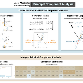
Perhaps the most basic type of unsupervised learning is dimension reduction methods, such as PCA, t-SNE, while PCA is generally used in data preprocessing, and t-SNE usually used in data visualization.
A more advanced branch is clustering, which explores the hidden patterns in data and then makes predictions on them; examples include K-mean clustering, Gaussian mixture models, hidden Markov models, and others.
Along with the renaissance of deep learning, unsupervised learning gains more and more attention because it frees us from manually labeling data. In light of deep learning, we consider two kinds of unsupervised learning: representation learning and generative models.
Representation learning aims to distill a high-level representative feature that is useful for some downstream tasks, while generative models intend to reproduce the input data from some hidden parameters.
To illustrate the example of unsupervised learning below | Source: Photo by Jelleke Vanooteghem, Unsplash
Unsupervised learning works as it sounds. In this type of algorithms, we do not have labeled data. So the machine has to process the input data and try to make conclusions about the output. For example, remember the kid whom we gave a shape toy? In this case, he would learn from its own mistakes to find the perfect shape hole for different shapes.
But the catch is that we are not feeding the child by teaching the methods to fit the shapes (for machine learning purposes called labeled data). However, the child learns from the toy’s different characteristics and tries to make conclusions about them. In short, the predictions are based on unlabeled data.
Examples of unsupervised learning algorithms:
Dimension Reduction
Density Estimation
Market Basket Analysis
Generative adversarial networks (GANs)
Clustering
What would a neural network look like in an abstract real-life example? | Source: Timo Volz, Unsplash
For this article, we will use a few types of regression algorithms with coding samples in Python.
1. Linear Regression:
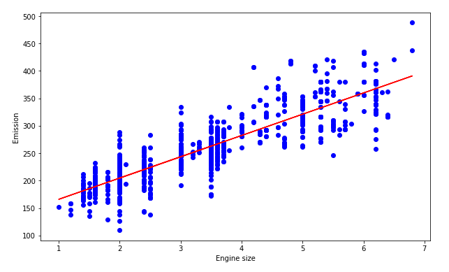
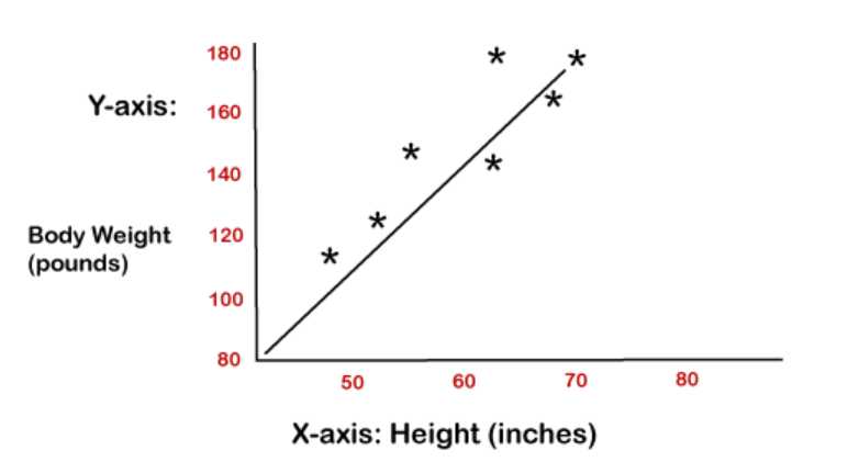
The Linear Regression algorithm in a graph | Source: Image processed with Python.
Linear regression is a statistical approach that models the relationship between input features and output. The input features are called the independent variables, and the output is called a dependent variable. Our goal here is to predict the value of the output based on the input features by multiplying it with its optimal coefficients.
Some real-life examples of linear regression :
(1) To predict sales of products.
(2) To predict economic growth.
(3) To predict petroleum prices.
(4) To predict the emission of a new car.
(5) Impact of GPA on college admissions.
There are two types of linear regression :
Simple Linear Regression
Multivariable Linear Regression
1.1 Simple Linear Regression:
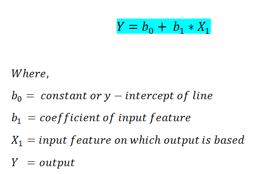
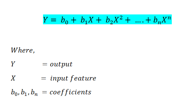
In simple linear regression, we predict the output/dependent variable based on only one input feature. The simple linear regression is given by:
Linear regression equation | Source: Image created by the author.
Below we are going to implement simple linear regression using the sklearn library in Python.
Step by step implementation in Python:
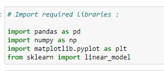
a. Import required libraries:
Since we are going to use various libraries for calculations, we need to import them.
Source: Image created by the author.
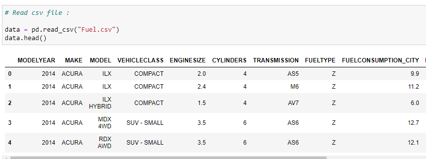
b. Read the CSV file:
Wecheck the first five rows of our dataset. In this case, we are using a vehicle model dataset — please check out the dataset on Softlayer IBM.
Source: Image created by the author.
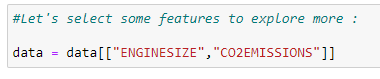
c. Select the features we want to consider in predicting values:
Here our goal is to predict the value of “co2 emissions” from the value of “engine size” in our dataset.
Source: Image created by the author.
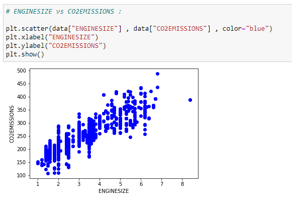
d. Plot the data:
We can visualize our data on a scatter plot.
Data plot for the linear regression algorithm | Source: Image created by the author.
e. Divide the data into training and testing data:
To check the accuracy of a model, we are going to divide our data into training and testing datasets. We will use training data to train our model, and then we will check the accuracy of our model using the testing dataset.
Source: Image created by the author.
f. Training our model:
Here is how we can train our model and find the coefficients for our best-fit regression line.
Source: Image created by the author.
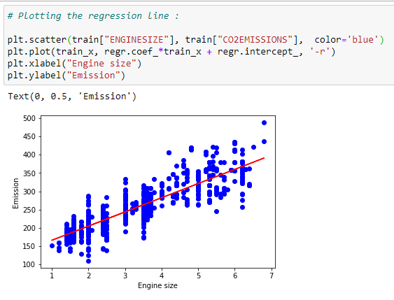
g. Plot the best fit line:
Based on the coefficients, we can plot the best fit line for our dataset.
Data plot for linear regression based on its coefficients | Source: Image created by the author.
h. Prediction function:
We are going to use a prediction function for our testing dataset.
Source: Image created by the author.
i. Predicting co2 emissions:
Predicting the values of co2 emissions based on the regression line.
Source: Image created by the author.
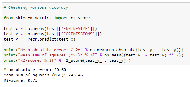
j. Checking accuracy for test data :
We can check the accuracy of a model by comparing the actual values with the predicted values in our dataset.
Source: Image created by the author.
Putting it all together:
# Import required libraries:
import pandas as pd
import numpy as np
import matplotlib.pyplot as plt
from sklearn import linear_model# Read the CSV file :
data = pd.read_csv(“Fuel.csv”)
data.head()# Let’s select some features to explore more :
data = data[[“ENGINESIZE”,”CO2EMISSIONS”]]# ENGINESIZE vs CO2EMISSIONS:
plt.scatter(data[“ENGINESIZE”] , data[“CO2EMISSIONS”] , color=”blue”)
plt.xlabel(“ENGINESIZE”)
plt.ylabel(“CO2EMISSIONS”)
plt.show()# Generating training and testing data from our data:
# We are using 80% data for training.
train = data[:(int((len(data)*0.8)))]
test = data[(int((len(data)*0.8))):]# Modeling:
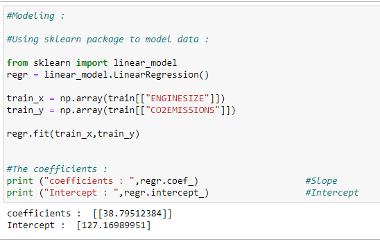
# Using sklearn package to model data :
regr = linear_model.LinearRegression()
train_x = np.array(train[[“ENGINESIZE”]])
train_y = np.array(train[[“CO2EMISSIONS”]])
regr.fit(train_x,train_y)# The coefficients:
print (“coefficients : “,regr.coef_) #Slope
print (“Intercept : “,regr.intercept_) #Intercept# Plotting the regression line:
plt.scatter(train[“ENGINESIZE”], train[“CO2EMISSIONS”], color=’blue’)
plt.plot(train_x, regr.coef_*train_x + regr.intercept_, ‘-r’)
plt.xlabel(“Engine size”)
plt.ylabel(“Emission”)# Predicting values:
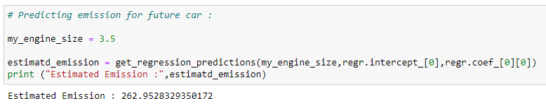
# Function for predicting future values :
def get_regression_predictions(input_features,intercept,slope):
predicted_values = input_features*slope + intercept
return predicted_values# Predicting emission for future car:
my_engine_size = 3.5
estimatd_emission = get_regression_predictions(my_engine_size,regr.intercept_[0],regr.coef_[0][0])
print (“Estimated Emission :”,estimatd_emission)# Checking various accuracy:
from sklearn.metrics import r2_score
test_x = np.array(test[[‘ENGINESIZE’]])
test_y = np.array(test[[‘CO2EMISSIONS’]])
test_y_ = regr.predict(test_x)print(“Mean absolute error: %.2f” % np.mean(np.absolute(test_y_ — test_y)))
print(“Mean sum of squares (MSE): %.2f” % np.mean((test_y_ — test_y) ** 2))
print(“R2-score: %.2f” % r2_score(test_y_ , test_y) )
1.2 Multivariable Linear Regression:
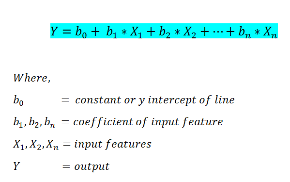
In simple linear regression, we were only able to consider one input feature for predicting the value of the output feature. However, in Multivariable Linear Regression, we can predict the output based on more than one input feature. Here is the formula for multivariable linear regression.
Multivariable linear regression equation | Source: Image created by the author.
Step by step implementation in Python:
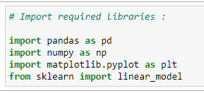
a. Import the required libraries:
Source: Image created by the author.
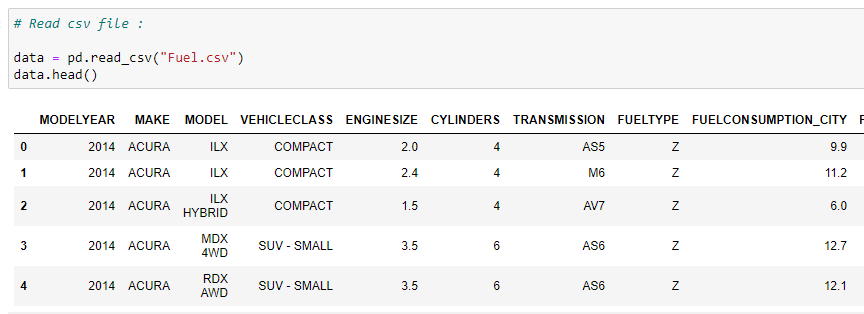
b. Read the CSV file :
Source: Image created by the author.
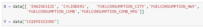
c. Define X and Y:
X stores the input features we want to consider, and Y stores the value of output.
Source: Image created by the author.
d. Divide data into a testing and training dataset:
Here we are going to use 80% data in training and 20% data in testing.
Source: Image created by the author.
e. Train our model :
Here we are going to train our model with 80% of the data.
Source: Image created by the author.
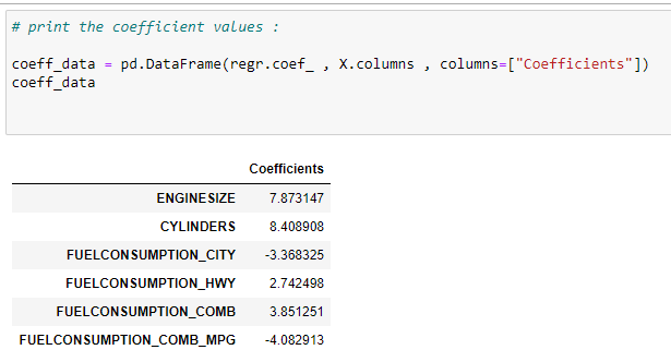
f. Find the coefficients of input features :
Now we need to know which feature has a more significant effect on the output variable. For that, we are going to print the coefficient values. Note that the negative coefficient means it has an inverse effect on the output. i.e., if the value of that features increases, then the output value decreases.
Source: Image created by the author.
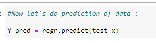
g. Predict the values:
Source: Image created by the author.
h. Accuracy of the model:
Source: Image created by the author.
Now notice that here we used the same dataset for simple and multivariable linear regression. We can notice that the accuracy of multivariable linear regression is far better than the accuracy of simple linear regression.
Putting it all together:
# Import the required libraries:
import pandas as pd
import numpy as np
import matplotlib.pyplot as plt
from sklearn import linear_model# Read the CSV file:
data = pd.read_csv(“Fuel.csv”)
data.head()# Consider features we want to work on:
X = data[[ ‘ENGINESIZE’, ‘CYLINDERS’, ‘FUELCONSUMPTION_CITY’,’FUELCONSUMPTION_HWY’,
‘FUELCONSUMPTION_COMB’,’FUELCONSUMPTION_COMB_MPG’]]Y = data[“CO2EMISSIONS”]# Generating training and testing data from our data:
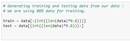
# We are using 80% data for training.
train = data[:(int((len(data)*0.8)))]
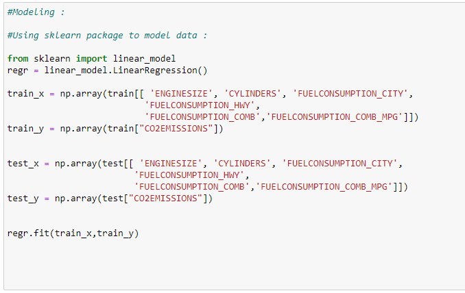
test = data[(int((len(data)*0.8))):]#Modeling:
#Using sklearn package to model data :
regr = linear_model.LinearRegression()train_x = np.array(train[[ ‘ENGINESIZE’, ‘CYLINDERS’, ‘FUELCONSUMPTION_CITY’,
‘FUELCONSUMPTION_HWY’, ‘FUELCONSUMPTION_COMB’,’FUELCONSUMPTION_COMB_MPG’]])
train_y = np.array(train[“CO2EMISSIONS”])regr.fit(train_x,train_y)test_x = np.array(test[[ ‘ENGINESIZE’, ‘CYLINDERS’, ‘FUELCONSUMPTION_CITY’,
‘FUELCONSUMPTION_HWY’, ‘FUELCONSUMPTION_COMB’,’FUELCONSUMPTION_COMB_MPG’]])
test_y = np.array(test[“CO2EMISSIONS”])# print the coefficient values:
coeff_data = pd.DataFrame(regr.coef_ , X.columns , columns=[“Coefficients”])
coeff_data#Now let’s do prediction of data:
Y_pred = regr.predict(test_x)# Check accuracy:
from sklearn.metrics import r2_score
R = r2_score(test_y , Y_pred)
print (“R² :”,R)
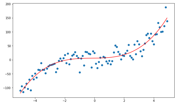
1.3 Polynomial Regression:
Source: Image created by the author.
Sometimes we have data that does not merely follow a linear trend. We sometimes have data that follows a polynomial trend. Therefore, we are going to use polynomial regression.
Before digging into its implementation, we need to know how the graphs of some primary polynomial data look.
Polynomial Functions and Their Graphs:
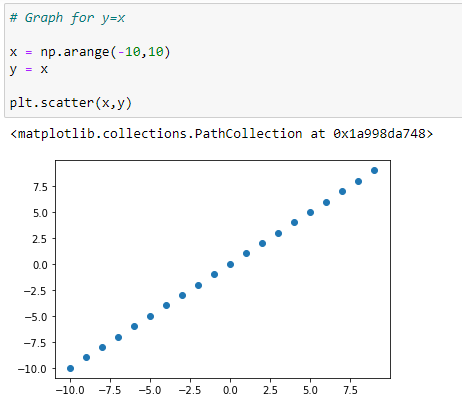
a. Graph for Y=X:
Source: Image created by the author.
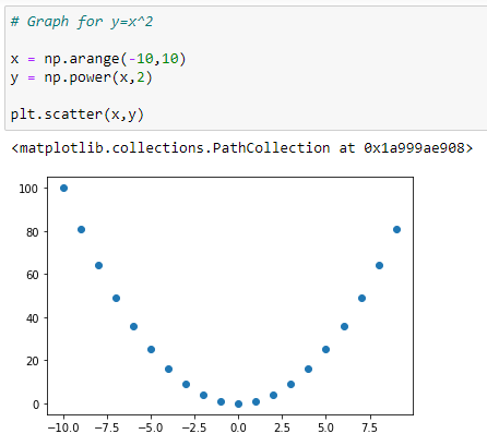
b. Graph for Y = X²:
Source: Image created by the author.
c. Graph for Y = X³:
Source: Image created by the author.
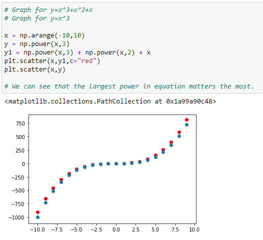
d. Graph with more than one polynomials: Y = X³+X²+X:
Source: Image created by the author.
In the graph above, we can see that the red dots show the graph for Y=X³+X²+X and the blue dots shows the graph for Y = X³. Here we can see that the most prominent power influences the shape of our graph.
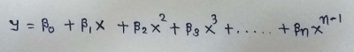
Below is the formula for polynomial regression:
The formula for a polynomial regression | Source: Image created by the author.
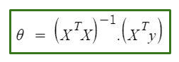
Now in the previous regression models, we used sci-kit learn library for implementation. Now in this, we are going to use Normal Equation to implement it. Here notice that we can use scikit-learn for implementing polynomial regression also, but another method will give us an insight into how it works.
The equation goes as follows:
Source: Image created by the author.
In the equation above:
θ: hypothesis parameters that define it the best.
X: input feature value of each instance.
Y: Output value of each instance.
1.3.1 Hypothesis Function for Polynomial Regression
Source: Image created by the author.
The main matrix in the standard equation:
Source: Image created by the author.
Step by step implementation in Python:
a. Import the required libraries:
Source: Image created by the author.
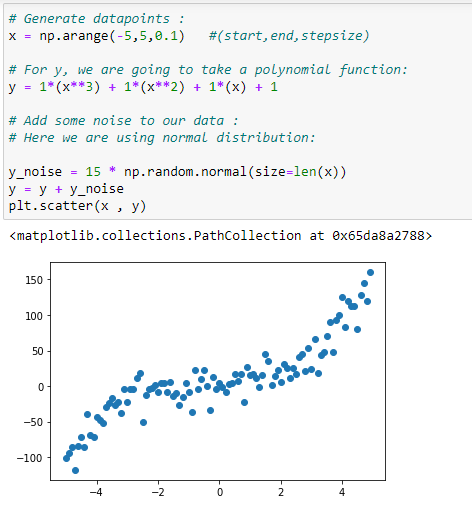
b. Generate the data points:
We are going to generate a dataset for implementing our polynomial regression.
Source: Image created by the author.
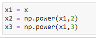
c. Initialize x,x²,x³ vectors:
We are taking the maximum power of x as 3. So our X matrix will have X, X², X³.
Source: Image created by the author.
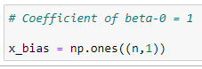
d. Column-1 of X matrix:
The 1st column of the main matrix X will always be 1 because it holds the coefficient of beta_0.
Source: Image created by the author.
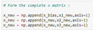
e. Form the complete x matrix:
Look at the matrix X at the start of this implementation. We are going to create it by appending vectors.
Source: Image created by the author.
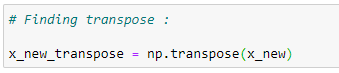
f. Transpose of the matrix:
We are going to calculate the value of theta step-by-step. First, we need to find the transpose of the matrix.
Source: Image created by the author.
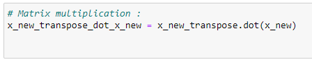
g. Matrix multiplication:
After finding the transpose, we need to multiply it with the original matrix. Keep in mind that we are going to implement it with a normal equation, so we have to follow its rules.
Source: Image created by the author.
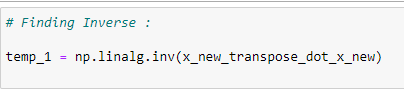
h. The inverse of a matrix:
Finding the inverse of the matrix and storing it in temp1.
Source: Image created by the author.
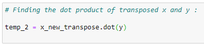
i. Matrix multiplication:
Finding the multiplication of transposed X and the Y vector and storing it in the temp2 variable.
Source: Image created by the author.
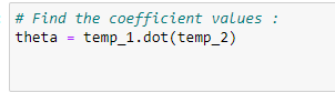
j. Coefficient values:
To find the coefficient values, we need to multiply temp1 and temp2. See the Normal Equation formula.
Source: Image created by the author.
k. Store the coefficients in variables:
Storing those coefficient values in different variables.
Source: Image created by the author.
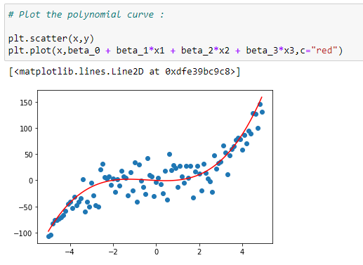
l. Plot the data with curve:
Plotting the data with the regression curve.
Source: Image created by the author.
m. Prediction function:
Now we are going to predict the output using the regression curve.
Source: Image created by the author.
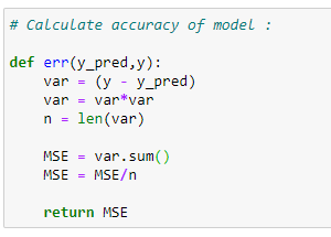
n. Error function:
Calculate the error using mean squared error function.
Source: Image created by the author.
o. Calculate the error:
Source: Image created by the author.
Putting it all together:
# Import required libraries:
import numpy as np
import matplotlib.pyplot as plt# Generate datapoints:
x = np.arange(-5,5,0.1)
y_noise = 20 * np.random.normal(size = len(x))
y = 1*(x**3) + 1*(x**2) + 1*x + 3+y_noise
plt.scatter(x,y)# Make polynomial data:
x1 = x
x2 = np.power(x1,2)
x3 = np.power(x1,3)# Reshaping data:
x1_new = np.reshape(x1,(n,1))
x2_new = np.reshape(x2,(n,1))
x3_new = np.reshape(x3,(n,1))# First column of matrix X:
x_bias = np.ones((n,1))# Form the complete x matrix:
x_new = np.append(x_bias,x1_new,axis=1)
x_new = np.append(x_new,x2_new,axis=1)
x_new = np.append(x_new,x3_new,axis=1)# Finding transpose:
x_new_transpose = np.transpose(x_new)# Finding dot product of original and transposed matrix :
x_new_transpose_dot_x_new = x_new_transpose.dot(x_new)# Finding Inverse:
temp_1 = np.linalg.inv(x_new_transpose_dot_x_new)# Finding the dot product of transposed x and y :
temp_2 = x_new_transpose.dot(y)# Finding coefficients:
theta = temp_1.dot(temp_2)
theta# Store coefficient values in different variables:
beta_0 = theta[0]
beta_1 = theta[1]
beta_2 = theta[2]
beta_3 = theta[3]# Plot the polynomial curve:
plt.scatter(x,y)
plt.plot(x,beta_0 + beta_1*x1 + beta_2*x2 + beta_3*x3,c=”red”)# Prediction function:
def prediction(x1,x2,x3,beta_0,beta_1,beta_2,beta_3):
 y_pred = beta_0 + beta_1*x1 + beta_2*x2 + beta_3*x3
 return y_pred

# Making predictions:
pred = prediction(x1,x2,x3,beta_0,beta_1,beta_2,beta_3)

# Calculate accuracy of model:
def err(y_pred,y):
 var = (y — y_pred)
 var = var*var
 n = len(var)
 MSE = var.sum()
 MSE = MSE/n

 return MSE# Calculating the error:
error = err(pred,y)
error
1.4 Exponential Regression:
Source: Image created by the author.
Some real-life examples of exponential growth:
1. Microorganisms in cultures.
2. Spoilage of food.
3. Human Population.
4. Compound Interest.
5. Pandemics (Such as Covid-19).
6. Ebola Epidemic.
7. Invasive Species.
8. Fire.
9. Cancer Cells.
10. Smartphone Uptake and Sale.
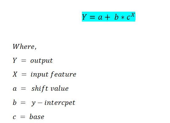
The formula for exponential regression is as follow:
The formula for the exponential regression | Source: Image created by the author.
In this case, we are going to use the scikit-learn library to find the coefficient values such as a, b, c.
Step by step implementation in Python
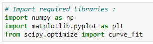
a. Import the required libraries:
Source: Image created by the author.
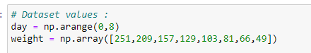
b. Insert the data points:
Source: Image created by the author.
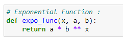
c. Implement the exponential function algorithm:
Source: Image created by the author.
d. Apply optimal parameters and covariance:
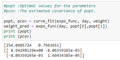
Here we use curve_fit to find the optimal parameter values. It returns two variables, called popt, pcov.
popt stores the value of optimal parameters, and pcov stores the values of its covariances. We can see that popt variable has two values. Those values are our optimal parameters. We are going to use those parameters and plot our best fit curve, as shown below.
Source: Image created by the author.
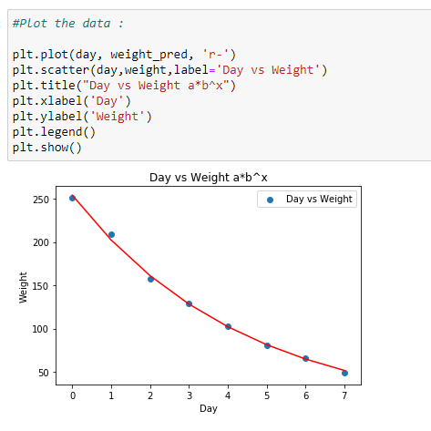
e. Plot the data:
Plotting the data with the coefficients found.
Source: Image created by the author.
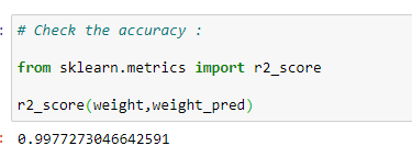
f. Check the accuracy of the model:
Check the accuracy of the model with r2_score.
Source: Image created by the author.
Putting it all together:
# Import required libraries:
import numpy as np
import matplotlib.pyplot as plt
from scipy.optimize import curve_fit# Dataset values :
day = np.arange(0,8)
weight = np.array([251,209,157,129,103,81,66,49])# Exponential Function :
def expo_func(x, a, b):
 return a * b ** x#popt :Optimal values for the parameters
#pcov :The estimated covariance of poptpopt, pcov = curve_fit(expo_func, day, weight)
weight_pred = expo_func(day,popt[0],popt[1])# Plotting the data
plt.plot(day, weight_pred, ‘r-’)
plt.scatter(day,weight,label=’Day vs Weight’)
plt.title(“Day vs Weight a*b^x”)
plt.xlabel(‘Day’)
plt.ylabel(‘Weight’)
plt.legend()
plt.show()# Equation
a=popt[0].round(4)
b=popt[1].round(4)
print(f’The equation of regression line is y={a}*{b}^x’
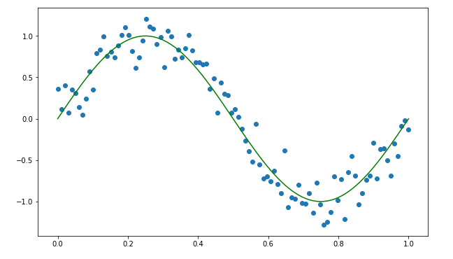
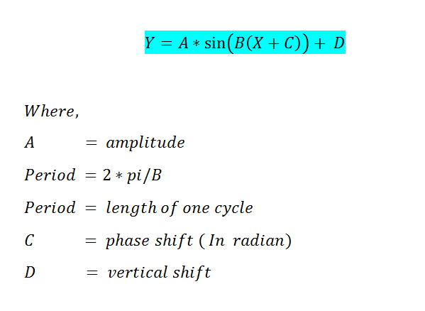
Sometimes we have data that shows patterns like a sine wave. Therefore, in such case scenarios, we use a sinusoidal regression. Below we can show the formula for the algorithm:
The formula for a sinusoidal regression | Source: Image created by the author.
Step by step implementation in Python:
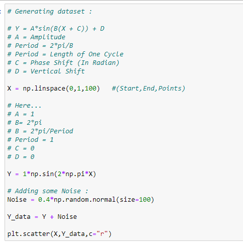
a. Generating the dataset:
Source: Image created by the author.Source: Image processed with Python.
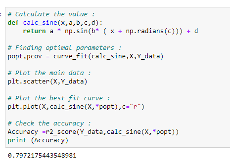
b. Applying a sine function:
Here we have created a function called “calc_sine” to calculate the value of output based on optimal coefficients. Here we will use the scikit-learn library to find the optimal parameters.
Source: Image created by the author.Source: Image processed with Python.
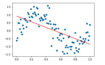
c. Why does a sinusoidal regression perform better than linear regression?
If we check the accuracy of the model after fitting our data with a straight line, we can see that the accuracy in prediction is less than that of sine wave regression. That is why we use sinusoidal regression.
Source: Image created by the author.Source: Image processed with Python.
Putting it all together:
# Import required libraries:
import numpy as np
import matplotlib.pyplot as plt
from scipy.optimize import curve_fit
from sklearn.metrics import r2_score# Generating dataset:# Y = A*sin(B(X + C)) + D
# A = Amplitude
# Period = 2*pi/B
# Period = Length of One Cycle
# C = Phase Shift (In Radian)
# D = Vertical ShiftX = np.linspace(0,1,100) #(Start,End,Points)# Here…
# A = 1
# B= 2*pi
# B = 2*pi/Period
# Period = 1
# C = 0
# D = 0Y = 1*np.sin(2*np.pi*X)# Adding some Noise :
Noise = 0.4*np.random.normal(size=100)Y_data = Y + Noiseplt.scatter(X,Y_data,c=”r”)# Calculate the value:
def calc_sine(x,a,b,c,d):
return a * np.sin(b* ( x + np.radians(c))) + d# Finding optimal parameters :
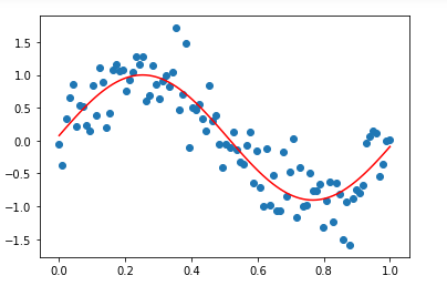
popt,pcov = curve_fit(calc_sine,X,Y_data)# Plot the main data :
plt.scatter(X,Y_data)# Plot the best fit curve :
plt.plot(X,calc_sine(X,*popt),c=”r”)# Check the accuracy :
Accuracy =r2_score(Y_data,calc_sine(X,*popt))
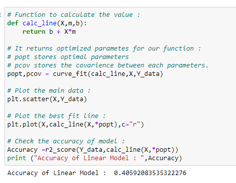
print (Accuracy)# Function to calculate the value :
def calc_line(X,m,b):
return b + X*m# It returns optimized parametes for our function :
# popt stores optimal parameters
# pcov stores the covarience between each parameters.
popt,pcov = curve_fit(calc_line,X,Y_data)# Plot the main data :
plt.scatter(X,Y_data)# Plot the best fit line :
plt.plot(X,calc_line(X,*popt),c=”r”)# Check the accuracy of model :
Accuracy =r2_score(Y_data,calc_line(X,*popt))
print (“Accuracy of Linear Model : “,Accuracy)
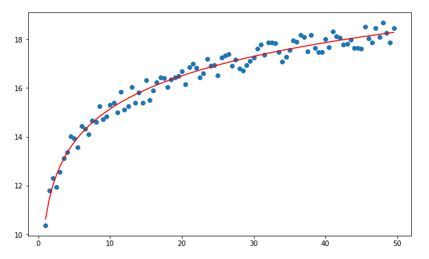
Graph for a logarithmic regression | Source: Image processed with Python.
Some real-life examples of logarithmic growth:
The magnitude of earthquakes.
The intensity of sound.
The acidity of a solution.
The pH level of solutions.
Yields of chemical reactions.
Production of goods.
Growth of infants.
A COVID-19 graph.
Sometimes we have data that grows exponentially in the statement, but after a certain point, it goes flat. In such a case, we can use a logarithmic regression.
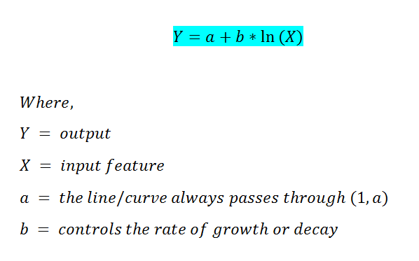
The equation for a logarithmic regression | Source: Image created by the author.
Step by step implementation in Python:
a. Import required libraries:
Source: Image created by the author.
b. Generating the dataset:
Source: Image created by the author.
c. The first column of our matrix X :
Here we will use our normal equation to find the coefficient values.
Source: Image created by the author.
d. Reshaping X:
Source: Image created by the author.
e. Going with the Normal Equation formula:
Source: Image created by the author.
f. Forming the main matrix X:
Source: Image created by the author.
g. Finding the transpose matrix:
Source: Image created by the author.
h. Performing matrix multiplication:
Source: Image created by the author.
i. Finding the inverse:
Source: Image created by the author.
j. Matrix multiplication:
Source: Image created by the author.
k. Finding the coefficient values:
Source: Image created by the author.
l. Plot the data with the regression curve:
Source: Image created by the author.
m. Accuracy:
Source: Image created by the author.
Putting it all together:
# Import required libraries:
import numpy as np
import matplotlib.pyplot as plt
from sklearn.metrics import r2_score# Dataset:
# Y = a + b*ln(X)
X = np.arange(1,50,0.5)
Y = 10 + 2*np.log(X)#Adding some noise to calculate error!
Y_noise = np.random.rand(len(Y))
Y = Y +Y_noise
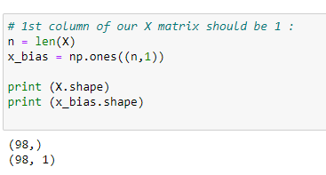
plt.scatter(X,Y)# 1st column of our X matrix should be 1:
n = len(X)
x_bias = np.ones((n,1))print (X.shape)
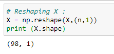
print (x_bias.shape)# Reshaping X :
X = np.reshape(X,(n,1))
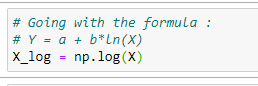
print (X.shape)# Going with the formula:
# Y = a + b*ln(X)
X_log = np.log(X)# Append the X_log to X_bias:
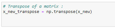
x_new = np.append(x_bias,X_log,axis=1)# Transpose of a matrix:
x_new_transpose = np.transpose(x_new)# Matrix multiplication:
x_new_transpose_dot_x_new = x_new_transpose.dot(x_new)# Find inverse:
temp_1 = np.linalg.inv(x_new_transpose_dot_x_new)# Matrix Multiplication:
temp_2 = x_new_transpose.dot(Y)# Find the coefficient values:
theta = temp_1.dot(temp_2)# Plot the data:
a = theta[0]
b = theta[1]
Y_plot = a + b*np.log(X)
plt.scatter(X,Y)
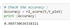
plt.plot(X,Y_plot,c=”r”)# Check the accuracy:
Accuracy = r2_score(Y,Y_plot)
print (Accuracy)
DISCLAIMER: The views expressed in this article are those of the author(s) and do not represent the views of Carnegie Mellon University, nor other companies (directly or indirectly) associated with the author(s). These writings do not intend to be final products, yet rather a reflection of current thinking, along with being a catalyst for discussion and improvement.
Citation
For attribution in academic contexts, please cite this work as:
Shukla, et al., “Machine Learning Algorithms For Beginners with Code Examples in Python”, Towards AI, 2020
BibTex citation:
@article{pratik_iriondo_chen_2020,
 title={Machine Learning Algorithms For Beginners with Code Examples in Python},
 url={https://towardsai.net/machine-learning-algorithms},
 journal={Towards AI},
 publisher={Towards AI Co.},
 author={Pratik, Shukla and Iriondo,
 Roberto and Chen, Sherwin},
 editor={Stanford, StacyEditor},
 year={2020},
 month={Jun}
}
What to consider before finalizing a Machine Learning algorithm?
The Principle behind Machine Learning Algorithms
Types of Machine Learning Algorithms
Most Used Machine Learning Algorithms – Explained
How to Choose Machine Learning Algorithms in Real Time
How to Run Machine Learning Algorithms?
Where do we stand in Machine Learning?
Applications of Machine Learning
Future of Machine Learning
Conclusion
The advancements in Science and Technology are making every step of our daily life more comfortable. Today, the use of Machine learning systems, which is an integral part of Artificial Intelligence, has spiked and is seen playing a remarkable role in every user’s life.
For instance, the widely popular, Virtual Personal Assistant being used for playing a music track or setting an alarm, face detection or voice recognition applications are awesome examples of the machine learning systems that we see every day. Here is an article on linear discriminant analysis for better understanding.
Machine learning, a subset of artificial intelligence, is the ability of a system to learn or predict the user’s needs and perform an expected task without human intervention. The inputs for the desired predictions are taken from user’s previously performed tasks or from relative examples. These are an example of practical machine learning with Python that makes prediction better.
Why Should You Choose Machine Learning?
Wonder why one should choose Machine Learning? Simply put, machine learning makes complex tasks much easier. It makes the impossible possible!
The following scenarios explain why we should opt for machine learning:
During facial recognition and speech processing, it would be tedious to write the codes manually to execute the process, that’s where machine learning comes handy.
For market analysis, figuring customer preferences or fraud detection, machine learning has become essential.
For the dynamic changes that happen in real-time tasks, it would be a challenging ordeal to solve through human intervention alone.
Essentials of Machine Learning Algorithms
To state simply, machine learning is all about predictions – a machine learning, thinking and predicting what’s next. Here comes the question – what will a machine learn, how will a machine analyze, what will it predict.
You have to understand two terms clearly before trying to get answers to these questions:
Data
Algorithm
Data
Data is what that is fed to the machine. For example, if you are trying to design a machine that can predict the weather over the next few days, then you should input the past ‘data’ that comprise maximum and minimum air temperatures, the speed of the wind, amount of rainfall, etc. All these come under ‘data’ that your machine will learn, and then analyse later.
If we observe carefully, there will always be some pattern or the other in the input data we have. For example, the maximum and minimum ranges of temperatures may fall in the same bracket; or speeds of the wind may be slightly similar for a given season, etc. But, machine learning helps analyse such patterns very deeply. And then it predicts the outcomes of the problem we have designed it for.
Algorithm
While data is the ‘food’ to the machine, an algorithm is like its digestive system. An algorithm works on the data. It crushes it; analyses it; permutates it; finds the gaps and fills in the blanks.
Algorithms are the methods used by machines to work on the data input to them. Learners must check if these concepts are being covered in the best data science courses they are enrolled in.
What to Consider Before Finalizing a Machine Learning Algorithm?
Depending on the functionality expected from the machine, algorithms range from very basic to highly complex. You should be wise in making a selection of an algorithm that suits your ML needs. Careful consideration and testing are needed before finalizing an algorithm for a purpose.
For example, linear regression works well for simple ML functions such as speech analysis. In case, accuracy is your first choice, then slightly higher level functionalities such as Neural networks will do.
This concept is called ‘The Explainability- Accuracy Tradeoff’. The following diagram explains this better:
Image Source
Besides, with regards to commonly used machine learning algorithms, you need to remember the following aspects very clearly:No algorithm is an all-in-one solution to any type of problem; an algorithm that fits a scenario is not destined to fit in another one.
Comparison of algorithms mostly does not make sense as each one of it has its own features and functionality. Many factors such as the size of data, data patterns, accuracy needed, the structure of the dataset, etc. play a major role in comparing two algorithms.
The Principle Behind Machine Learning Algorithms
As we learnt, an algorithm churns the given data and finds a pattern among them. Thus, all machine learning algorithms, especially the ones used for supervised learning, follow one similar principle:
If the input variables or the data is X and you expect the machine to give a prediction or output Y, the machine will work on as per learning a target function ‘f’, whose pattern is not known to us.
Thus, Y= f(X) fits well for every supervised machine learning algorithm. This is otherwise also called Predictive Modeling or Predictive Analysis, which ultimately provides us with the best ever prediction possible with utmost accuracy.
Types of Machine Learning Algorithms
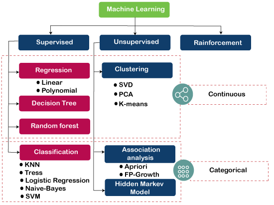
Diving further into machine learning, we will first discuss the types of algorithms it has. Machine learning algorithms can be classified as:
Supervised, and
Unsupervised
Semi-supervised algorithms
Reinforcement algorithms
A brief description of the types of algorithms is given below:
1. Supervised machine learning algorithms
In this method, to get the output for a new set of user’s input, a model is trained to predict the results by using an old set of inputs and its relative known set of outputs. In other words, the system uses the examples used in the past.
A data scientist trains the system on identifying the features and variables it should analyze. After training, these models compare the new results to the old ones and update their data accordingly to improve the prediction pattern.
An example: If there is a basket full of fruits, based on the earlier specifications like color, shape and size given to the system, the model will be able to classify the fruits.
There are 2 techniques in supervised machine learning and a technique to develop a model is chosen based on the type of data it has to work on.
A) Techniques used in Supervised learning
Supervised algorithms use either of the following techniques to develop a model based on the type of data.
Regression
Classification
1. Regression Technique
In a given dataset, this technique is used to predict a numeric value or continuous values (a range of numeric values) based on the relation between variables obtained from the dataset.
An example would be guessing the price of a house based after a year, based on the current price, total area, locality and number of bedrooms.
Another example is predicting the room temperature in the coming hours, based on the volume of the room and current temperature.
2. Classification Technique
This is used if the input data can be categorized based on patterns or labels.
For example, an email classification like recognizing a spam mail or face detection which uses patterns to predict the output.
In summary, the regression technique is to be used when predictable data is in quantity and Classification technique is to be used when predictable data is about predicting a label.
B) Algorithms that use Supervised Learning
Some of the machine learning algorithms which use supervised learning method are:
Linear Regression
Logistic Regression
Random Forest
Gradient Boosted Trees
Support Vector Machines (SVM)
Neural Networks
Decision Trees
Naive Bayes
We shall discuss some of these algorithms in detail as we move ahead in this post.
2. Unsupervised machine learning algorithms
This method does not involve training the model based on old data, I.e. there is no “teacher” or “supervisor” to provide the model with previous examples.
The system is not trained by providing any set of inputs and relative outputs. Instead, the model itself will learn and predict the output based on its own observations.
For example, consider a basket of fruits which are not labeled/given any specifications this time. The model will only learn and organize them by comparing Color, Size and shape.
A. Techniques used in unsupervised learning
We are discussing these techniques used in unsupervised learning as under:
Clustering
Dimensionality Reduction
Anomaly detection
Neural networks
1. Clustering
It is the method of dividing or grouping the data in the given data set based on similarities.
Data is explored to make groups or subsets based on meaningful separations.
Clustering is used to determine the intrinsic grouping among the unlabeled data present.
An example where clustering principle is being used is in digital image processing where this technique plays its role in dividing the image into distinct regions and identifying image border and the object.
2. Dimensionality reduction
In a given dataset, there can be multiple conditions based on which data has to be segmented or classified.
These conditions are the features that the individual data element has and may not be unique.
If a dataset has too many numbers of such features, it makes it a complex process to segregate the data.
To solve such type of complex scenarios, dimensional reduction technique can be used, which is a process that aims to reduce the number of variables or features in the given dataset without loss of important data.
This is done by the process of feature selection or feature extraction.
Email Classification can be considered as the best example where this technique was used.
3. Anomaly Detection
Anomaly detection is also known as Outlier detection.
It is the identification of rare items, events or observations which raise suspicions by differing significantly from the majority of the data.
Examples of the usage are identifying a structural defect, errors in text and medical problems.
4. Neural Networks
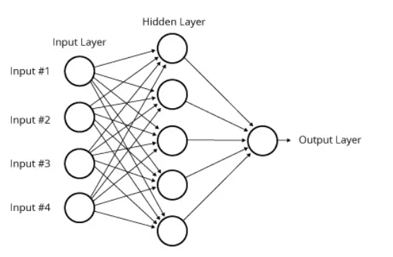
A Neural network is a framework for many different machine learning algorithms to work together and process complex data inputs.
It can be thought of as a “complex function” which gives some output when an input is given.
The Neural Network consists of 3 parts which are needed in the construction of the model.
Units or Neurons
Connections or Parameters.
Biases.
Neural networks are into a wide range of applications such as coastal engineering, hydrology and medicine where they are being used in identifying certain types of cancers.
B. Algorithms that use unsupervised learning
Some of the most common algorithms in unsupervised learning are:
hierarchical clustering,
k-means
mixture models
DBSCAN
OPTICS algorithm
Autoencoders
Deep Belief Nets
Hebbian Learning
Generative Adversarial Networks
Self-organizing map
We shall discuss some of these algorithms in detail as we move ahead in this post.
3.Semi Supervised Algorithms
In case of semi-supervised algorithms, as the name goes, it is a mix of both supervised and unsupervised algorithms. Here both labelled and unlabelled examples exist, and in many scenarios of semi-supervised learning, the count of unlabelled examples is more than that of labelled ones.
Classification and regression form typical examples for semi-supervised algorithms.
The algorithms under semi-supervised learning are mostly extensions of other methods, and the machines that are trained in the semi-supervised method make assumptions when dealing with unlabelled data.
Examples of Semi Supervised Learning:
Google Photos are the best example of this model of learning. You must have observed that at first, you define the user name in the picture and teach the features of the user by choosing a few photos. Then the algorithm sorts the rest of the pictures accordingly and asks you in case it gets any doubts during classification.
Comparing with the previous supervised and unsupervised types of learning models, we can make the following inferences for semi-supervised learning:
Labels are entirely present in case of supervised learning, while for unsupervised learning they are totally absent. Semi-supervised is thus a hybrid mix of both these two.
The semi-supervised model fits well in cases where cost constraints are present for machine learning modelling. One can label the data as per cost requirements and leave the rest of the data to the machine to take up.
Another advantage of semi-supervised learning methods is that they have the potential to exploit the unlabelled data of a group in cases where data carries important unexploited information.
4. Reinforcement Learning
In this type of learning, the machine learns from the feedback it has received. It constantly learns and upgrades its existing skills by taking the feedback from the environment it is in.
Markov’s Decision process is the best example of reinforcement learning.
In this mode of learning, the machine learns iteratively the correct output. Based on the reward obtained from each iteration,the machine knows what is right and what is wrong. This iteration keeps going till the full range of probable outputs are covered.
Process of Reinforcement Learning
The steps involved in reinforcement learning are as shown below:
Input state is taken by the agent
A predefined function indicates the action to be performed
Based on the action, the reward is obtained by the machine
The resulting pair of feedback and action is stored for future purposes
Examples of Reinforcement Learning Algorithms
Computer based games such as chess
Artificial hands that are based on robotics
Driverless cars/ self-driven cars
Most Used Machine Learning Algorithms – Explained
In this section, let us discuss the following most widely used machine learning algorithms in detail:
Decision Trees
Naive Bayes Classification
The Autoencoder
Self-organizing map
Hierarchical clustering
OPTICS algorithm
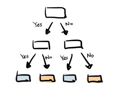
1. Decision Trees
This algorithm is an example of supervised learning.
A Decision tree is a pictorial representation or a graphical representation which depicts every possible outcome of a decision.
The various elements involved here are node, branch and leaf where ‘node’ represents an ‘attribute’, ‘branch’ representing a ‘decision’ and ‘leaf’ representing an ‘outcome’ of the feature after applying that particular decision.
A decision tree is just an analogy of how a human thinks to take a decision with yes/no questions.
The below decision tree explains a school admission procedure rule, where Age is primarily checked, and if age is < 5, admission is not given to them. And for the kids who are eligible for admission, a check is performed on Annual income of parents where if it is < 3 L p.a. the students are further eligible to get a concession on the fees.
2. Naive Bayes Classification
This supervised machine learning algorithm is a powerful and fast classifying algorithm, using the Bayes rule in determining the conditional probability and to predict the results.
Its popular uses are, face recognition, filtering spam emails, predicting the user inputs in chat by checking communicated text and to label news articles as sports, politics etc.
Bayes Rule: The Bayes theorem defines a rule in determining the probability of occurrence of an “Event” when information about “Tests” is provided.
“Event” can be considered as the patient having a Heart disease while “tests” are the positive conditions that match with the event
3. The Autoencoder
It comes under the category of unsupervised learning using neural networking techniques.
An autoencoder is intended to learn or encode a representation for a given data set.
This also involves the process of dimensional reduction which trains the network to remove the “noise” signal.
In hand, with the reduction, it also works in reconstruction where the model tries to rebuild or generate a representation from the reduced encoding which is equivalent to the original input.
I.e. without the loss of important and needed information from the given input, an Autoencoder removes or ignores the unnecessary noise and also works on rebuilding the output.
Pic source
The most common use of Autoencoder is an application that converts black and white image to color. Based on the content and object in the image (like grass, water, sky, face, dress) coloring is processed.
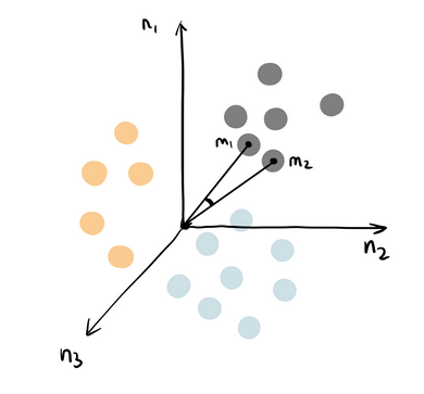
4. Self-organizing map
This comes under the unsupervised learning method.
Self-Organizing Map uses the data visualization technique by operating on a given high dimensional data.
The Self-Organizing Map is a two-dimensional array of neurons: M = {m1,m2,……mn}
It reduces the dimensions of the data to a map, representing the clustering concept by grouping similar data together.
SOM reduces data dimensions and displays similarities among data.
SOM uses clustering technique on data without knowing the class memberships of the input data where several units compete for the current object.
In short, SOM converts complex, nonlinear statistical relationships between high-dimensional data into simple geometric relationships on a low-dimensional display.
5. Hierarchical clustering
Hierarchical clustering uses one of the below clustering techniques to determine a hierarchy of clusters.
Thus produced hierarchy resembles a tree structure which is called a “Dendrogram”.
The techniques used in hierarchical clustering are:
K-Means,
DBSCAN,
Gaussian Mixture Models.
The 2 methods in finding hierarchical clusters are:
Agglomerative clustering
Divisive clustering
Agglomerative clustering
This is a bottom-up approach, where each data point starts in its own cluster.
These clusters are then joined greedily, by taking the two most similar clusters together and merging them.
Divisive clustering
Inverse to Agglomerative, this uses a top-down approach, wherein all data points start in the same cluster after which a parametric clustering algorithm like K-Means is used to divide the cluster into two clusters.
Each cluster is further divided into two clusters until a desired number of clusters are hit.
6. OPTICS algorithm
OPTICS is an abbreviation for ordering points to identify the clustering structure.
OPTICS works in principle like an extended DB Scan algorithm for an infinite number for a distance parameter which is smaller than a generating distance.
From a wide range of parameter settings, OPTICS outputs a linear list of all objects under analysis in clusters based on their density.
How to Choose Machine Learning Algorithms in Real Time
When implementing algorithms in real time, you need to keep in mind three main aspects: Space, Time, and Output.
Besides, you should clearly understand the aim of your algorithm:
Do you want to make predictions for the future?
Are you just categorizing the given data?
Is your targeted task simple or comprises of multiple sub-tasks?
The following table will show you certain real-time scenarios and help you to understand which algorithm is best suited to each scenario:
Real time scenario
Best suited algorithm
Why this algorithm is the best fit?
Simple straightforward data set with no complex computations
Linear Regression
It takes into account all factors involved and predicts the result with simple error rate explanation.For simple computations, you need not spend much computational power; and linear regression runs with minimal computational power.
Classifying already labeled data into sub-labels
Logistic Regression
This algorithm looks at every data point into two subcategories, hence best for sub-labeling.Logistic regression model works best when you have multiple targets.
Sorting unlabelled data into groups
K-Means clustering algorithm
This algorithm groups and clusters data by measuring the spatial distance between each point.You can choose from its sub-types – Mean-Shift algorithm and Density-Based Spatial Clustering of Applications with Noise
Supervised text classification (analyzing reviews, comments, etc.)
Naive Bayes
Simplest model that can perform powerful pre-processing and cleaning of textRemoves filler stop words effectivelyComputationally in-expensive
Logistic regression
Sorts words one by one and assigns a probabilityRanks next to Naïve Bayes in simplicity
Linear Support Vector Machine algorithm
Can be chosen when performance matters
Bag-of-words model
Suits best when vocabulary and the measure of known words is known.
Image classification
Convolutional neural network
Best suited for complex computations such as analyzing visual cortexesConsumes more computational power and gives the best results
Stock market predictions
Recurrent neural network
Best suited for time-series analysis with well-defined and supervised data.Works efficiently in taking into account the relation between data and its time distribution.
How to Run Machine Learning Algorithms?
Till now you have learned in detail about various algorithms of machine learning, their features, selection and application in real time.
When implementing the algorithm in real time, you can do it in any programming language that works well for machine learning.
All that you need to do is use the standard libraries of the programming language that you have chosen and work on them, or program everything from scratch.
Need more help? You can check these links for more clarity on coding machine learning algorithms in various programming languages.
How To Get Started With Machine Learning Algorithms in R
How to Run Your First Classifier in Weka
Machine Learning Algorithm Recipes in scikit-learn
Where do We Stand in Machine Learning?
Machine learning is slowly making strides into as many fields in our daily life as possible. Some businesses are making it strict to have transparent algorithms that do not affect their business privacy or data security. They are even framing regulations and performing audit trails to check if there is any discrepancy in the above-said data policies.
The point to note here is that a machine working on machine learning principles and algorithms give output after processing the data through many nonlinear computations. If one needs to understand how a machine predicts, perhaps it can be possible only through another machine learning algorithm!
Applications of Machine Learning
Currently, the role of Machine learning and Artificial Intelligence in human life is intertwined. With the advent of evolving technologies, AI and ML have marked their existence in all possible aspects.
Machine learning finds a plethora of applications in several domains of our day to day life. An exhaustive list of fields where machine learning is currently in use now is shown in the diagram here. An explanation for the same follows further below:
Financial Services: Banks and financial services are increasingly relying on machine learning to identify financial fraud, portfolio management, identify and suggest good options for investment for customers.
Police Department: Apps based on facial recognition and other techniques of machine learning are being used by the police to identify and get hold of criminals.
Online Marketing and Sales: Machine learning is helping companies a great deal in studying the shopping and spending patterns of customers and in making personalized product recommendations to them. Machine learning also eases customer support, product recommendations and advertising ideas for e-commerce.
Healthcare: Doctors are using machine learning to predict and analyze the health status and disease progress of patients. Machine learning has proven its accuracy in detecting health condition, heartbeat, blood pressure and in identifying certain types of cancer. Advanced techniques of machine learning are being implemented in robotic surgery too.
Household Applications: Household appliances that use face detection and voice recognition are gaining popularity as security devices and personal virtual assistants at homes.
Oil and Gas: In analyzing underground minerals and carrying out the exploration and mining, geologists and scientists are using machine learning for improved accuracy and reduced investments.
Transport: Machine learning can be used to identify the vehicles that are moving in prohibited zones for traffic control and safety monitoring purposes.
Social Media: In social media, spam is a big nuisance. Companies are using machine learning to filter spam. Machine learning also aptly solves the purpose of sentiment analysis in social media.
Trading and Commerce: Machine learning techniques are being implemented in online trading to automate the process of trading. Machines learn from the past performances of trading and use this knowledge to make decisions about future trading options.
Future of Machine Learning
Machine learning is already making a difference in the way businesses are offering their services to us, the customers. Voice-based search and preferences based ads are just basic functionalities of how machine learning is changing the face of businesses.
ML has already made an inseparable mark in our lives. With more advancement in various fields, ML will be an integral part of all AI systems. ML algorithms are going to be made continuously learning with the day-to-day updating information.
With the rapid rate at which ongoing research is happening in this field, there will be more powerful machine learning algorithms to make the way we live even more sophisticated!
From 2013- 2017, the patents in the field of machine learning has recorded a growth of 34%, according to IFI Claims Patent Services (Patent Analytics). Also, 60% of the companies in the world are using machine learning for various purposes.
A peek into the future trends and growth of machine learning through the reports of Predictive Analytics and Machine Learning (PAML) market shows a 21% CAGR by 2021.
Conclusion
Ultimately, machine learning should be designed as an aid that would support mankind. The notion that automation and machine learning are threats to jobs and human workforce is pretty prevalent. It should always be remembered that machine learning is just a technology that has evolved to ease the life of humans by reducing the needed manpower and to offer increased efficiency at lower costs that too in a shorter time span. The onus of using machine learning in a responsible manner lies in the hands of those who work on/with it.
However, stay tuned to an era of artificial intelligence and machine learning that makes the impossible possible and makes you witness the unseen! Want to execute what you have learned in this blog, enroll in KnowledgeHut practical machine learning with Python and work with data science projects that deal with complex machine learning algorithms.
Machine Learning came a long way from a science fiction fancy to a reliable and diverse business tool that amplifies multiple elements of the business operation.
Its influence on business performance may be so significant that the implementation of machine learning algorithms is required to maintain competitiveness in many fields and industries.
The implementation of machine learning in business operations is a strategic step and requires a lot of resources. Therefore, it’s important to understand what do you want the ML to do for your particular business and what kind of perks different types of ML algorithms bring to the table.
In this article, we’ll cover the major types of machine learning algorithms, explain the purpose of each of them, and see what the benefits are.
PREDICTIVE ANALYTICS VS. MACHINE LEARNING: WHAT IS THE DIFFERENCE
Types of Machine Learning Algorithms
Algorithms include supervised and unsupervised learning systems as well as Reinforcement and Semi-supervised machine learning technology.
Supervised Learning Algorithms
Supervised Learning Algorithms are the ones that involve direct supervision (cue the title) of the operation. In this case, the developer labels sample data corpus and set strict boundaries upon which the algorithm operates.
It is a spoonfed version of machine learning:
you select what kind of information output (samples) to “feed” the algorithm;
what kind of results it is desired (for example “yes/no” or “true/false”).
From the machine’s point of view, this process becomes more or less a “connect the dots” routine.
The primary purpose of supervised learning is to scale the scope of input data and to make predictions of unavailable, future or unseen data based on labeled sample data.
Supervised machine learning includes two major processes: classification and regression.
Classification is the process where incoming data is labeled based on past data samples and manually trains the algorithm to recognize certain types of objects and categorize them accordingly. The system has to know how to differentiate types of information, perform an optical character, image, or binary recognition (whether a particular bit of data is compliant or non-compliant to specific requirements in a manner of “yes” or “no”).
Regression is the process of identifying patterns and calculating the predictions of continuous outcomes. The system has to understand the numbers, their values, grouping (for example, heights and widths), etc.
The most widely used supervised algorithms are:
Linear Regression
Logistical Regression
Random Forest
Gradient Boosted Trees
Support Vector Machines (SVM)
Neural Networks
Decision Trees
Naive Bayes
Nearest Neighbor
Supervised Learning Algorithms Use Cases
The most common fields of use for supervised learning algorithm is price prediction and trend forecasting in sales, retail commerce, and stock trading. In both cases, an algorithm uses incoming data to assess the possibility and calculate possible outcomes.
The best examples are Sales enablement platforms like Seismic and Highspot use this kind of an algorithm to present various possible scenarios for consideration.
Business cases for supervised learning method include ad tech operations as part of the ad content delivery sequence. The role of the supervised learning system there is to assess possible prices of ad spaces and its value during the real-time bidding process and also keep the budget spending under specific limitations (for example, the price range of a single buy and overall budget for a certain period).
Unsupervised Learning Algorithms
Unsupervised Learning is one that does not involve direct control of the developer. If the main point of supervised machine learning is that you know the results and need to sort out the new data, then in the case of unsupervised learning algorithm the desired results are unknown and yet to be defined.
Another big difference between the two is that supervised learning uses labeled data exclusively, while unsupervised learning feeds on unlabeled data.
The unsupervised machine learning algorithm is used for:
exploring the structure of the information;
extracting valuable insights;
detecting patterns;
implementing this into its operation to increase efficiency.
In other words, unsupervised learning techniques describe information by sifting through it and making sense of it.
Unsupervised learning algorithms apply the following techniques to describe the data:
Clustering: it is an exploration of data used to segment it into meaningful groups (i.e., clusters) based on their internal patterns without prior knowledge of group credentials. The credentials are defined by the similarity of individual data objects and also aspects of their dissimilarity from the rest (which can also be used to detect anomalies).
Dimensionality reduction: there is a lot of noise in the incoming data. Machine learning algorithms use dimensionality reduction to remove this noise while distilling the relevant information.
Digital marketing and ad tech are the fields where unsupervised learning is used to its maximum effect. In addition to that, this algorithm is often applied to explore customer information and adjust the service accordingly.
The thing is – there are a lot of so-called “known unknowns” in the incoming data. The very effectiveness of the business operation depends on the ability to make sense of unlabeled data and extract relevant insights out of it.
Unsupervised algorithms equip modern data management. At the moment, Lotame and Salesforce are among the most cutting-edge data management platforms that implement this machine learning system.
As such, unsupervised learning can be used to identify target audience groups based on certain credentials (it can be behavioral data, elements of personal data, specific software setting or else). This algorithm can be used to develop more efficient targeting of ad content and also for identifying patterns in the campaign performance.
Semi-supervised Machine Learning Algorithms
Semi-supervised learning algorithms represent a middle ground between supervised and unsupervised algorithms. In essence, the semi-supervised model combines some aspects of both into a thing of its own.
Here’s how semi-supervised algorithms work:
A semi-supervised machine-learning algorithm uses a limited set of labeled sample data to shape the requirements of the operation (i.e., train itself).
The limitation results in a partially trained model that later gets the task to label the unlabeled data. Due to the limitations of the sample data set, the results are considered pseudo-labeled data.
Finally, labeled and pseudo-labeled data sets are combined, which creates a distinct algorithm that combines descriptive and predictive aspects of supervised and unsupervised learning.
Semi-supervised learning uses the classification process to identify data assets and the clustering process to group it into distinct parts.
Semi-supervised Machine Learning Use Cases
Legal and Healthcare industries, among others, manage web content classification, image, and speech analysis with the help of semi-supervised learning.
In the case of web content classification, semi-supervised learning is applied for crawling engines and content aggregation systems. In both cases, it uses a wide array of labels to analyze content and arrange it in specific configurations. However, this procedure usually requires human input for further classification.
An excellent example of this will be uClassify. The other well-known tool of this category is the GATE (General Architecture for Text Engineering).
In the case of image and speech analysis, an algorithm performs labeling to provide a viable image or speech analytic model with coherent transcription based on a sample corpus. For example, it can be an MRI or CT scan. With a small set of exemplary scans, it is possible to provide a coherent model able to identify anomalies in the images.
Reinforcement Learning Algorithms
Reinforcement learning represents what is commonly understood as machine learning artificial intelligence.
In essence, reinforcement learning is all about developing a self-sustained system that, throughout contiguous sequences of tries and fails, improves itself based on the combination of labeled data and interactions with the incoming data.
Reinforced ML uses the technique called exploration/exploitation. The mechanics are simple – the action takes place, the consequences are observed, and the next action considers the results of the first action.
In the center of reinforcement learning algorithms are reward signals that occur upon performing specific tasks. In a way, reward signals are serving as a navigation tool for the reinforcement algorithms. They give it an understanding of right and wrong course of action.
Two main types of reward signals are:
Positive reward signal encourages continuing performance a particular sequence of action
Negative reward signal penalizes for performing certain activities and urges to correct the algorithm to stop getting penalties.
However, the function of the reward signal may vary depending on the nature of the information. Thus reward signals may be further classified depending on the requirements of the operation. Overall, the system tries to maximize positive rewards and minimize the negatives.
Most common reinforcement learning algorithms include:
Q-Learning
Temporal Difference (TD)
Monte-Carlo Tree Search (MCTS)
Asynchronous Actor-Critic Agents (A3C)
TOP AI USE CASES IN SUPPLY CHAIN OPTIMIZATION
Use Cases for Reinforced Machine Learning Algorithms
Reinforcement Machine Learning fits for instances of limited or inconsistent information available. In this case, an algorithm can form its operating procedures based on interactions with data and relevant processes.
Modern NPCs and other video games use this type of machine learning model a lot. Reinforcement Learning provides flexibility to the AI reactions to the player’s action thus providing viable challenges. For example, the collision detection feature uses this type of ML algorithm for the moving vehicles and people in the Grand Theft Auto series.
Self-driving cars also rely on reinforced learning algorithms as well. For example, if the self-driving car (Waymo, for instance) detects the road turn to the left – it may activate the “turn left” scenario and so on.
The most famous example of this variation of reinforcement learning is AlphaGo that went head to head with the second-best Go player in the world and outplayed him by calculating the sequences of actions out of current board position.
On the other hand, Marketing and Ad Tech operations also use Reinforcement Learning. This type of machine learning algorithm can make retargeting operation much more flexible and efficient in delivering conversion by closely adapting to the user’s behavior and surrounding context.
Also, Reinforcement learning is used to amplify and adjust natural language processing (NLP) and dialogue generation for chatbots to:
mimic the style of an input message
develop more engaging, informative kinds of responses
find relevant responses according to the user reaction.
With the emergence of Google DialogFlow building, such bot became more of a UX challenge than a technical feat.
What do we think about ML intelligent algorithm?
As you can see, different types of machine learning algorithms are solving different kinds of problems. The combination of different algorithms makes a power capable of handling a wide variety of tasks and extracting valuable insights out of all sorts of information.
Whether your business is a taxi app or a food delivery service or even a social media network – every app can benefit from machine learning algorithms. Ready to begin? The APP Solutions team has expertise in architecting and implementing ML algorithms into various types of projects and we’d love to see your business grow.
Machine learning (ML) algorithms are computer programs that adapt and evolve based on the data they process to produce predetermined outcomes. They are essentially mathematical models that “learn” by being fed data—often referred to as “training data.” Common types of ML algorithms include linear regression and decision trees. Practical applications of ML algorithms include fraud detection and the automatic delivery of personalized marketing offers in retail.
Broadly speaking, there are two main categories of ML algorithms: supervised and unsupervised ML. Supervised ML algorithms involve “teaching” the machine to produce outputs based on its training data, which is already labelled or structured. Unsupervised ML algorithms, on the other hand, work with unstructured data—data that hasn’t already been classified or labeled.
Why Do Machine Learning Algorithms Matter?
ML is the most widely used and fastest-growing subset of AI today. Used to improve a wide array of computing concepts, including computer programming itself, it is often referred to as Software 2.0.
ML algorithms are integrated into just about every kind of device and hardware, from smartphones to servers to watches and sensors. They are increasingly the backbone behind many technological innovations and benefits, from ridesharing to autonomous vehicles to spam filtering, and many more.
Supervised vs. Unsupervised vs. Reinforcement Learning
The easiest way to distinguish a supervised learning and unsupervised learning is to see whether the data is labelled or not.
Supervised learning learns a function to make prediction of a defined label based on the input data. It can be either classifying data into a category (classification problem) or forecasting an outcome (regression algorithms).
Unsupervised learning reveals the underlying pattern in the dataset that are not explicitly presented, which can discover the similarity of data points (clustering algorithms) or uncover hidden relationships of variables (association rule algorithms) …
Reinforcement learning is another type of machine learning, where the agents learn to take actions based on its interaction with the environment, with the aim to maximize rewards. It is most similar to the learning process of human, following a trial-and-error approach.
Classification vs Regression
Supervised learning can be furthered categorized into classification and regression algorithms. Classification model identifies which category an object belongs to whereas regression model predicts a continuous output.
For a guide to regression algorithms, please see:
Top 4 Regression Algorithms in Machine Learning
A Comprehensive Guide to Implementation and Comparison
Sometimes there is an ambiguous line between classification algorithms and regression algorithms. Many algorithms can be used for both classification and regression, and classification is just regression model with a threshold applied. When the number is higher than the threshold it is classified as true while lower classified as false.
In this article, we will discuss top 6 machine learning algorithms for classification problems, including: logistic regression, decision tree, random forest, support vector machine, k nearest neighbour and naive bayes. I summarized the theory behind each as well as how to implement each using python. Check out the code for model pipeline on my website.
1. Logistic Regression
logistic regression (image by author)
Logistics regression uses sigmoid function above to return the probability of a label. It is widely used when the classification problem is binary — true or false, win or lose, positive or negative …
The sigmoid function generates a probability output. By comparing the probability with a pre-defined threshold, the object is assigned to a label accordingly. Check out my posts on logistic regression for a detailed walkthrough.
Simple Logistic Regression in Python
Step-by-Step Guide from Data Preprocessing to Model Evaluation
Below is the code snippet for a default logistic regression and the common hyperparameters to experiment on — see which combinations bring the best result.
logistic regression common hyperparameters: penalty, max_iter, C, solver
2. Decision Tree
decision tree (image by author)
Decision tree builds tree branches in a hierarchy approach and each branch can be considered as an if-else statement. The branches develop by partitioning the dataset into subsets based on most important features. Final classification happens at the leaves of the decision tree.
decision tree common hyperparameters: criterion, max_depth, min_samples_split, min_samples_leaf; max_features
3. Random Forest
random forest (image by author)
As the name suggest, random forest is a collection of decision trees. It is a common type of ensemble methods which aggregate results from multiple predictors. Random forest additionally utilizes bagging technique that allows each tree trained on a random sampling of original dataset and takes the majority vote from trees. Compared to decision tree, it has better generalization but less interpretable, because of more layers added to the model.
random forest common hyperparameters: n_estimators, max_features, max_depth, min_samples_split, min_samples_leaf, boostrap
4. Support Vector Machine (SVM)
support vector machine (image by author)
Support vector machine finds the best way to classify the data based on the position in relation to a border between positive class and negative class. This border is known as the hyperplane which maximize the distance between data points from different classes. Similar to decision tree and random forest, support vector machine can be used in both classification and regression, SVC (support vector classifier) is for classification problem.
support vector machine common hyperparameters: c, kernel, gamma
5. K-Nearest Neighbour (KNN)
knn (image by author)
You can think of k nearest neighbour algorithm as representing each data point in a n dimensional space — which is defined by n features. And it calculates the distance between one point to another, then assign the label of unobserved data based on the labels of nearest observed data points. KNN can also be used for building recommendation system, check out my article on “Collaborative Filtering for Movie Recommendation” if you are interested in this topic.
KNN common hyperparameters: n_neighbors, weights, leaf_size, p
6. Naive Bayes
naive bayes (image by author)
Naive Bayes is based on Bayes’ Theorem — an approach to calculate conditional probability based on prior knowledge, and the naive assumption that each feature is independent to each other. The biggest advantage of Naive Bayes is that, while most machine learning algorithms rely on large amount of training data, it performs relatively well even when the training data size is small. Gaussian Naive Bayes is a type of Naive Bayes classifier that follows the normal distribution.
I chose the popular dataset Heart Disease UCI on Kaggle for predicting the presence of heart disease based on several health related factors.
Use df.info()to have a summarized view of dataset, including data type, missing data and number of records.
2. Exploratory Data Analysis (EDA)
Histogram, grouped bar chart and box plot are suitable EDA techniques for classification machine learning algorithms. If you’d like a more comprehensive guide to EDA, please see my post “Semi-Automated Exploratory Data Analysis Process in Python”
Semi-Automated Exploratory Data Analysis Process in Python
This article covers several techniques to automate the EDA process using Python, including univariate analysis
Univariate Analysis
univariate analysis (image by author)
Histogram is used for all features, because all features have been encoded into numeric values in the dataset. This saves us the time for categorical encoding that usually happens during the feature engineering stage.
Categorical Features vs. Target — Grouped Bar Chart
grouped bar chart (image by author)
To show how categorical value weigh in determining the target value, grouped bar chart is a straightforward representation. For example, sex = 1 and sex = 0 have distinctly distribution of target value, which indicates it is likely to contribute more to the prediction of target. Contrarily, if the target distribution is the same regardless of the categorical features, then very likely they are not correlated.
Numerical Features vs. Target — Box Plot
box plot (image by author)
Box plot shows how the values of numerical features varies across target groups. For example, we can tell that “oldpeak” have distinct difference when target is 0 vs. target is 1, suggesting that it is an important predictor. However, ‘trestbps’ and ‘chol’ appear to be less outstanding, as the box plot distribution is similar between target groups.
3. Split Dataset into Training and Testing Set
Classification algorithm falls under the category of supervised learning, so dataset needs to be split into a subset for training and a subset for testing (sometime also a validation set). The model is trained on the training set and then examined using the testing set.
from sklearn.model_selection import train_test_split
from sklearn import preprocessingX = df.drop(['target'], axis=1)
y = df["target"]X_train, X_test, y_train, y_test = train_test_split(X, y, test_size=0.33, random_state=42)
4. Machine Learning Model Pipeline
In order to create a pipeline, I append the default state of all classification algorithms mentioned above into the model list and then iterate through them to train, test, predict and evaluate.
model pipeline (image by author)
5. Model Evaluation
model evaluation (image by author)
Below is an abstraction explanation of commonly used evaluation methods for classification models — accuracy, ROC & AUC and confusion matrix. Each of the following metrics is worth diving deeper, feel free to visit my article on logistic regression for a more detailed illustration.
1. Accuracy
Accuracy is the most straightforward indicator of the model performance. It measure the percentage of accurate predictions: accuracy = (true positive + true negative) / (true positive + false positive + false negative + false positive)
2. ROC & AUC
ROC & AUC (image by author)
ROC is the plot of true positive rate against false positive rate at various classification threshold. AUC is the area under the ROC curve, and higher AUC indicates better model performance.
3. Confusion matrix
Confusion matrix indicates the actual values vs. predicted values and summarize the true negative, false positive, false negative and true positive values in a matrix format.
Then we can use seaborn to visualize the confusion matrix in a heatmap.
confusion matrix plot (image by author)accuracy and AUC result (image by author)
Based on three evaluations methods above, random forests and naive bayes have the best performance, whereas KNN is not doing well. However, this doesn’t mean that random forests and naive bayes are superior algorithms. We can only say that they are more suitable for this dataset where the size is relatively smaller and data is not at the same scale.
Each algorithm has its own preference and require different data processing and feature engineering techniques, for example KNN is sensitive to features at difference scale and multicollinearity affects the result of logistic regression. Understanding the characteristics of each allows us to balance the trade-off and select the appropriate model according to the dataset.
Thanks for reaching so far, if you’d like to read more articles from Medium and also support my work, I really appreciate you signing up Medium Membership using this affiliate link.
Take Home Message
This article is an introduction of following 6 machine learning algorithms and a guide to build a model pipeline to address classification problems:
Machine Learning algorithms are the programs that can learn the hidden patterns from the data, predict the output, and improve the performance from experiences on their own. Different algorithms can be used in machine learning for different tasks, such as simple linear regression that can be used for prediction problems like stock market prediction, and the KNN algorithm can be used for classification problems.
In this topic, we will see the overview of some popular and most commonly used machine learning algorithms along with their use cases and categories.
Types of Machine Learning Algorithms
Machine Learning Algorithm can be broadly classified into three types:
Supervised Learning Algorithms
Unsupervised Learning Algorithms
Reinforcement Learning algorithm
The below diagram illustrates the different ML algorithm, along with the categories:
1) Supervised Learning Algorithm
Supervised learning is a type of Machine learning in which the machine needs external supervision to learn. The supervised learning models are trained using the labeled dataset. Once the training and processing are done, the model is tested by providing a sample test data to check whether it predicts the correct output.
The goal of supervised learning is to map input data with the output data. Supervised learning is based on supervision, and it is the same as when a student learns things in the teacher’s supervision. The example of supervised learning is spam filtering.
Supervised learning can be divided further into two categories of problem:
Classification
Regression
Examples of some popular supervised learning algorithms are Simple Linear regression, Decision Tree, Logistic Regression, KNN algorithm, etc.
2) Unsupervised Learning Algorithm
It is a type of machine learning in which the machine does not need any external supervision to learn from the data, hence called unsupervised learning. The unsupervised models can be trained using the unlabelled dataset that is not classified, nor categorized, and the algorithm needs to act on that data without any supervision. In unsupervised learning, the model doesn’t have a predefined output, and it tries to find useful insights from the huge amount of data. These are used to solve the Association and Clustering problems. Hence further, it can be classified into two types:
Clustering
Association
Examples of some Unsupervised learning algorithms are K-means Clustering, Apriori Algorithm, Eclat, etc.
3) Reinforcement Learning
In Reinforcement learning, an agent interacts with its environment by producing actions, and learn with the help of feedback. The feedback is given to the agent in the form of rewards, such as for each good action, he gets a positive reward, and for each bad action, he gets a negative reward. There is no supervision provided to the agent. Q-Learning algorithm is used in reinforcement learning.
List of Popular Machine Learning Algorithm
Linear Regression Algorithm
Logistic Regression Algorithm
Decision Tree
SVM
Naïve Bayes
KNN
K-Means Clustering
Random Forest
Apriori
PCA
1. Linear Regression
Linear regression is one of the most popular and simple machine learning algorithms that is used for predictive analysis. Here, predictive analysis defines prediction of something, and linear regression makes predictions for continuous numbers such as salary, age, etc.
It shows the linear relationship between the dependent and independent variables, and shows how the dependent variable(y) changes according to the independent variable (x).
It tries to best fit a line between the dependent and independent variables, and this best fit line is knowns as the regression line.
The equation for the regression line is:
y= a0+ a*x+ b
Here, y= dependent variable
x= independent variable
a0 = Intercept of line.
Linear regression is further divided into two types:
Simple Linear Regression: In simple linear regression, a single independent variable is used to predict the value of the dependent variable.
Multiple Linear Regression: In multiple linear regression, more than one independent variables are used to predict the value of the dependent variable.
2. Logistic Regression
Logistic regression is the supervised learning algorithm, which is used to predict the categorical variables or discrete values. It can be used for the classification problems in machine learning, and the output of the logistic regression algorithm can be either Yes or NO, 0 or 1, Red or Blue, etc.
Logistic regression is similar to the linear regression except how they are used, such as Linear regression is used to solve the regression problem and predict continuous values, whereas Logistic regression is used to solve the Classification problem and used to predict the discrete values.
Instead of fitting the best fit line, it forms an S-shaped curve that lies between 0 and 1. The S-shaped curve is also known as a logistic function that uses the concept of the threshold. Any value above the threshold will tend to 1, and below the threshold will tend to 0.
3. Decision Tree Algorithm
A decision tree is a supervised learning algorithm that is mainly used to solve the classification problems but can also be used for solving the regression problems. It can work with both categorical variables and continuous variables. It shows a tree-like structure that includes nodes and branches, and starts with the root node that expand on further branches till the leaf node. The internal node is used to represent the features of the dataset, branches show the decision rules, and leaf nodes represent the outcome of the problem.
Some real-world applications of decision tree algorithms are identification between cancerous and non-cancerous cells, suggestions to customers to buy a car, etc.
4. Support Vector Machine Algorithm
A support vector machine or SVM is a supervised learning algorithm that can also be used for classification and regression problems. However, it is primarily used for classification problems. The goal of SVM is to create a hyperplane or decision boundary that can segregate datasets into different classes.
The data points that help to define the hyperplane are known as support vectors, and hence it is named as support vector machine algorithm.
Some real-life applications of SVM are face detection, image classification, Drug discovery, etc. Consider the below diagram:
As we can see in the above diagram, the hyperplane has classified datasets into two different classes.
5. Naïve Bayes Algorithm:
Naïve Bayes classifier is a supervised learning algorithm, which is used to make predictions based on the probability of the object. The algorithm named as Naïve Bayes as it is based on Bayes theorem, and follows the naïve assumption that says’ variables are independent of each other.
The Bayes theorem is based on the conditional probability; it means the likelihood that event(A) will happen, when it is given that event(B) has already happened. The equation for Bayes theorem is given as:
Naïve Bayes classifier is one of the best classifiers that provide a good result for a given problem. It is easy to build a naïve bayesian model, and well suited for the huge amount of dataset. It is mostly used for text classification.
6. K-Nearest Neighbour (KNN)
K-Nearest Neighbour is a supervised learning algorithm that can be used for both classification and regression problems. This algorithm works by assuming the similarities between the new data point and available data points. Based on these similarities, the new data points are put in the most similar categories. It is also known as the lazy learner algorithm as it stores all the available datasets and classifies each new case with the help of K-neighbours. The new case is assigned to the nearest class with most similarities, and any distance function measures the distance between the data points. The distance function can be Euclidean, Minkowski, Manhattan, or Hamming distance, based on the requirement.
7. K-Means Clustering
K-means clustering is one of the simplest unsupervised learning algorithms, which is used to solve the clustering problems. The datasets are grouped into K different clusters based on similarities and dissimilarities, it means, datasets with most of the commonalties remain in one cluster which has very less or no commonalities between other clusters. In K-means, K-refers to the number of clusters, and means refer to the averaging the dataset in order to find the centroid.
It is a centroid-based algorithm, and each cluster is associated with a centroid. This algorithm aims to reduce the distance between the data points and their centroids within a cluster.
This algorithm starts with a group of randomly selected centroids that form the clusters at starting and then perform the iterative process to optimize these centroids’ positions.
It can be used for spam detection and filtering, identification of fake news, etc.
8. Random Forest Algorithm
Random forest is the supervised learning algorithm that can be used for both classification and regression problems in machine learning. It is an ensemble learning technique that provides the predictions by combining the multiple classifiers and improve the performance of the model.
It contains multiple decision trees for subsets of the given dataset, and find the average to improve the predictive accuracy of the model. A random-forest should contain 64-128 trees. The greater number of trees leads to higher accuracy of the algorithm.
To classify a new dataset or object, each tree gives the classification result and based on the majority votes, the algorithm predicts the final output.
Random forest is a fast algorithm, and can efficiently deal with the missing & incorrect data.
9. Apriori Algorithm
Apriori algorithm is the unsupervised learning algorithm that is used to solve the association problems. It uses frequent itemsets to generate association rules, and it is designed to work on the databases that contain transactions. With the help of these association rule, it determines how strongly or how weakly two objects are connected to each other. This algorithm uses a breadth-first search and Hash Tree to calculate the itemset efficiently.
The algorithm process iteratively for finding the frequent itemsets from the large dataset.
The apriori algorithm was given by the R. Agrawal and Srikant in the year 1994. It is mainly used for market basket analysis and helps to understand the products that can be bought together. It can also be used in the healthcare field to find drug reactions in patients.
10. Principle Component Analysis
Principle Component Analysis (PCA) is an unsupervised learning technique, which is used for dimensionality reduction. It helps in reducing the dimensionality of the dataset that contains many features correlated with each other. It is a statistical process that converts the observations of correlated features into a set of linearly uncorrelated features with the help of orthogonal transformation. It is one of the popular tools that is used for exploratory data analysis and predictive modeling.
PCA works by considering the variance of each attribute because the high variance shows the good split between the classes, and hence it reduces the dimensionality.
Some real-world applications of PCA are image processing, movie recommendation system, optimizing the power allocation in various communication channels.
In recent years, the field of machine learning has made significant advances in different problem types, from image recognition to natural language processing.
However, most of these models operate on data from a single modality, such as images, text, or speech. In contrast, real-world data often comes from multiple modalities, such as images and text, video and audio, or sensor data from multiple sources.
To address this challenge, researchers have developed multimodal machine learning models that can handle data from multiple modalities, unlocking new possibilities for intelligent systems.
In this blog post, we will explore the challenges and opportunities of multimodal machine learning, and discuss the different architectures and techniques used to tackle multimodal computer vision challenges.
What is Multimodal Deep Learning?
Multimodal Deep Learning is a subset of deep learning that deals with the fusion and analysis of data from multiple modalities, such as text, images, video, audio, and sensor data. Multimodal Deep Learning combines the strengths of different modalities to create a more complete representation of the data, leading to better performance on various machine learning tasks.
Traditionally, machine learning models were designed to work on data from a single modality, such as image classification or speech recognition. However, in the real world, data often comes from multiple sources and modalities, making it more complex and difficult to analyze. Multimodal Deep Learning aims to overcome this challenge by integrating information from different modalities to generate more accurate and informative models.
What is the Goal of Multimodal Deep Learning?
The primary goal of Multimodal Deep Learning is to create a shared representation space that can effectively capture complementary information from different modalities. This shared representation can then be used to perform various tasks, such as image captioning, speech recognition, and natural language processing.
Multimodal Deep Learning models typically consist of multiple neural networks, each specialized in analyzing a particular modality. The output of these networks is then combined using various fusion techniques, such as early fusion, late fusion, or hybrid fusion, to create a joint representation of the data.
Early fusion involves concatenating the raw data from different modalities into a single input vector and feeding it to the network. Late fusion, on the other hand, involves training separate networks for each modality and then combining their outputs at a later stage. Hybrid fusion combines elements of both early and late fusion to create a more flexible and adaptable model.
How Does Multimodal Learning Work?
Multimodal deep learning models are typically composed of multiple unimodal neural networks, which process each input modality separately. For instance, an audiovisual model may have two unimodal networks, one for audio and another for visual data. This individual processing of each modality is known as encoding.
Once unimodal encoding is done, the information extracted from each modality must be integrated or fused. There are several fusion techniques available, ranging from simple concatenation to attention mechanisms. Multimodal data fusion is a critical factor for the success of these models. Finally, a “decision” network accepts the fused encoded information and is trained on the task at hand.
In general, multimodal architectures consist of three parts:
Unimodal encoders encode individual modalities. Usually, one for each input modality.
A fusion network that combines the features extracted from each input modality, during the encoding phase.
A classifier that accepts the fused data and makes predictions.
Pictured: A general multimodal workflow. It involves several unimodal neural networks (three in this case) to independently encode various input modalities. The extracted features are then combined using a fusion module. Finally, the fused features are fed into a classification network to make the prediction.
Encoding Stage
The encoder extracts features from the input data in each modality and converts them into a common representation that can be processed by subsequent layers in the model. The encoder is typically composed of several layers of neural networks that use nonlinear transformations to extract increasingly abstract features from the input data.
The input to the encoder can consist of data from multiple modalities, such as images, audio, and text, which are typically processed separately. Each modality has its own encoder that transforms the input data into a set of feature vectors. The output of each encoder is then combined into a single representation that captures the relevant information from each modality.
One popular approach for combining the outputs of the individual encoders is to concatenate them into a single vector. Another approach is to use attention mechanisms to weigh the contributions of each modality based on their relevance to the task at hand.
The overall goal of the encoder is to capture the underlying structure and relationships between the input data from multiple modalities, enabling the model to make more accurate predictions or generate new outputs based on this multimodal input.
Fusion Module
The fusion module combines information from different modalities (e.g., text, image, audio) into a single representation that can be used for downstream tasks such as classification, regression, or generation. The fusion module can take various forms depending on the specific architecture and task at hand
One common approach is to use a weighted sum of the modalities’ features, where the weights are learned during training. Another approach is to concatenate the modalities’ features and pass them through a neural network to learn a joint representation.
In some cases, attention mechanisms can be used to learn which modality should be attended to at each time step.
Regardless of the specific implementation, the goal of the fusion module is to capture the complementary information from different modalities and create a more robust and informative representation for the downstream task. This is especially important in applications such as video analysis, where combining visual and audio cues can greatly improve performance.
Classification
The classification module takes the joint representation generated by the fusion module and uses it to make a prediction or decision. The specific architecture and approach used in the classification module can vary depending on the task and type of data being processed.
In many cases, the classification module takes the form of a neural network, where the joint representation is passed through one or more fully connected layers before the final prediction is made. These layers can include non-linear activation functions, dropout, and other techniques to help prevent overfitting and improve generalization performance.
The output of the classification module depends on the specific task at hand. For example, in a multimodal sentiment analysis task, the output will be a binary decision indicating whether the text and image input is positive or negative. In a multimodal image captioning task, the output might be a sentence describing the content of the image.
The classification module is typically trained using a supervised learning approach, where the input modalities and their corresponding labels or targets are used to optimize the parameters of the model. This optimization is often done using gradient-based optimization methods such as stochastic gradient descent or its variants.
In review, the classification module plays a critical role in multimodal deep learning by taking the joint representation generated by the fusion module and using it to make an informed decision or prediction.
Multimodal Learning in Computer Vision
In recent years, multimodal learning has emerged as a promising approach to tackle complex computer vision tasks by combining information from multiple modalities such as images, text, and speech.
This approach has enabled significant progress in several areas, including:
Visual question answering;
Text-to-image generation, and;
Natural language for visual reasoning.
In this section, we will explore how multimodal learning models have revolutionized computer vision and made it possible to achieve impressive results in challenging tasks that previously seemed impossible. Specifically, we will dive into the workings of three popular uses of multimodal architectures in the computer vision field: Visual Question Answering (VQA), Text-to-Image Generation, and Natural Language for Visual Reasoning (NLVR).
Visual Question Answering (VQA)
Visual Question Answering (VQA) involves answering questions based on visual input, such as images or videos, using natural language. VQA is a challenging task that requires a deep understanding of both computer vision and natural language processing.
In recent years, VQA has seen significant progress due to the use of deep learning techniques and architectures, particularly the Transformer architecture. The Transformer architecture was originally introduced for language processing tasks and has shown great success in VQA.
One of the most successful models for VQA is the PaLI (Pathways Language and Image model) model developed by Google Research in 2022. PaLI architecture uses an encoder-decoder Transformer model, with a large-capacity ViT component for image processing.
PaLI model architecture.
Text-to-Image Generation
In text-to-image generation, a machine learning model is trained to generate images based on textual descriptions. The goal is to create a system that can understand natural language and use that understanding to generate visual content that accurately represents the meaning of the input text.https://www.youtube.com/embed/LM8dil6n5h8?feature=oembed
The two most recent and successful models are DALL-E and Stable Diffusion.
DALL-E is a text-to-image generation model developed by OpenAI, which uses a combination of a transformer-based language model and a generative neural network architecture. The model takes in a textual description and generates an image that satisfies the description. DALL-E can generate a wide variety of complex and creative images, such as a snail made of harps and a collage of a red tree kangaroo in a field of daisies.
One of the key innovations in DALL-E is the use of a discrete latent space, which allows the model to learn a more structured and controllable representation of the generated images. DALL-E is trained on a large dataset of image-text pairs, and the model is optimized using a variant of the VAE loss function called the Gumbel-Softmax trick.
The Stable Diffusion architecture is a recent technique for generating high-quality images based on text prompts. Stable Diffusion uses a diffusion process, which involves iteratively adding noise to an initial image and then progressively removing the noise.
By controlling the level of noise and the number of iterations, Stable Diffusion can generate diverse and high-quality images that match the input text prompt.
The key innovation in Stable Diffusion is the use of a diffusion process that allows for stable and diverse image generation. In addition, diffusion uses a contrastive loss function to encourage the generated images to be diverse and distinct from each other. Diffusion has achieved impressive results in text-to-image generation, and it can generate high-quality images that closely match the input text prompts.
Natural Language for Visual Reasoning (NLVR)
Natural Language for Visual Reasoning (NLVR) aims to evaluate the ability of models to understand and reason about natural language descriptions of visual scenes. In this task, a model is given a textual description of a scene and two corresponding images, one of which is consistent with the description and the other not. The objective of the model is to identify the correct image that matches the given textual description.
NLVR requires the model to understand complex linguistic structures and reason about visual information to make the correct decision. The task involves a variety of challenges, such as understanding spatial relations, recognizing objects and their properties, and understanding the semantics of natural language.
The current state-of-the-art on the NLVR task is reached by BEiT-3. It is a transformer-based model that has been pre-trained on large-scale datasets of natural images and texts, such as ImageNet and Conceptual Captions.
BEiT-3 architecture for a NLVR task.
BEiT-3 is designed to handle both natural language and visual information and is capable of reasoning about complex linguistic structures and visual scenes.
The architecture of BEiT-3 is similar to that of other transformer-based models, such as BERT and GPT, but with some modifications to handle visual data. The model consists of an encoder and a decoder, where the encoder takes in both the visual and textual inputs and the decoder produces the output.
Challenges Building Multimodal Model Architectures
Multimodal Deep Learning has revolutionized the way we approach complex data analysis tasks, such as image and speech recognition. However, working with data from multiple modalities poses unique challenges that must be addressed to achieve optimal performance.
In this section, we will discuss some of the key challenges associated with Multimodal Deep Learning.
Alignment
Alignment is the process of ensuring that data from different modalities are synchronized or aligned in time, space, or any other relevant dimension. The lack of alignment between modalities can lead to inconsistent or incomplete representations, which can negatively impact the performance of the model.
Alignment can be particularly challenging in scenarios where the modalities are acquired at different times or from different sources. A prime example of a situation where alignment is a difficult challenge to solve is in video analysis. Aligning the audio with the visual information can be challenging due to the latency introduced by the data acquisition process. Similarly, in speech recognition, aligning the audio with the corresponding transcription can be difficult due to variations in speaking rates, accents, and background noise.
Several techniques have been proposed to address the alignment challenge in multimodal machine learning models. For instance, temporal alignment methods can be used to align the data in time by estimating the time offset between modalities. Spatial alignment methods can be used to align data in space by identifying corresponding points or features in different modalities.
Additionally, deep learning techniques, such as attention mechanisms, can be used to automatically align the data during the model training process. However, each alignment technique has its strengths and limitations, and the choice of alignment method depends on the specific problem and the characteristics of the data.
Co-learning
Co-learning involves jointly learning from multiple modalities to improve the performance of the model. In co-learning, the model learns from the correlations and dependencies between the different modalities, which can lead to a more robust and accurate representation of the underlying data.
Co-learning requires designing models that can handle the heterogeneity and variability of the data from different modalities, while also identifying the relevant information that can be shared across modalities. This is challenging. Additionally, co-learning can lead to the problem of negative transfer, where learning from one modality negatively impacts the performance of the model on another modality.
To address the co-learning challenge in multimodal machine learning models, several techniques have been proposed. One approach is to use joint representation learning methods, such as deep canonical correlation analysis (DCCA) or cross-modal deep metric learning (CDML), which aim to learn a shared representation that captures the correlations between the modalities. Another approach is to use attention mechanisms that can dynamically allocate the model’s resources to the most informative modalities or features.
Co-learning is still an active research area in multimodal machine learning, and there are many open questions and challenges to be addressed, such as how to handle missing modalities or how to incorporate prior knowledge into the learning process.
Translation
Translation involves converting the data from one modality or language to another. For example, translating speech to text, text to speech, or image to text.
Multimodal machine learning models that require translation must take into account the differences in the structure, syntax, and semantics between the source and target languages or modalities. Additionally, they must be able to handle the variability in the input data, such as different accents or dialects, and adapt to the context of the input.
There are several approaches to address the translation challenge in multimodal machine learning models. One common approach is to use neural machine translation (NMT) models, which have shown great success in translating text from one language to another. NMT models can also be used to translate speech to text or vice versa by training on paired audio-text data. Another approach is to use multimodal models that can learn to map data from one modality to another, such as image-to-text or speech-to-text translation.
However, translating between modalities or languages is a challenging task. The performance of the translation models heavily depends on the quality and size of the training data, the complexity of the task, and the availability of computing resources.
Fusion
Fusion involves combining information from different modalities to make a decision or prediction. There are different ways to fuse data, including early fusion, late fusion, and hybrid fusion.
Early fusion involves combining the raw data from different modalities at the input level. This approach requires aligning and pre-processing the data, which can be challenging due to differences in data formats, resolutions, and sizes.
Late fusion, on the other hand, involves processing each modality separately and then combining the outputs at a later stage. This approach can be more robust to differences in data formats and modalities, but it can also lead to the loss of important information.
Hybrid fusion is a combination of both early and late fusion approaches, where some modalities are fused at the input level, while others are fused at a later stage.
Choosing the appropriate fusion method is critical to the success of a multimodal machine learning model. The fusion method must be tailored to the specific problem and the characteristics of the data. Additionally, the fusion method must be designed to preserve the most relevant information from each modality and avoid the introduction of noise or irrelevant information.
Conclusion
Multimodal Deep Learning is an exciting and rapidly evolving field that holds great potential for advancing computer vision and other areas of artificial intelligence.
Through the integration of multiple modalities, including visual, textual, and auditory information, multimodal learning allows machines to perceive and interpret the world around them in ways that were once only possible for humans.
In this post, we highlighted three key applications of multimodal learning in computer vision: Visual Question Answering, Text-to-Image Generation, and Natural Language for Visual Reasoning.
While there are challenges associated with multimodal learning, including the need for large amounts of training data and the difficulty of fusing information from multiple modalities, recent advances in deep learning models have led to significant improvements in performance across a range of tasks.
Machine Learning algorithms are being used more often than we can imagine and there is a good reason for that.
Let’s see what kind of different Machine Learning algorithms exist and how they can help us in solving everyday life problems.
Machine Learning is not the future. It’s the present
Many different Machine Learning algorithms are widely used in many areas of our life and they help us to solve some everyday problems. Algorithms can help us not only to recognize images, videos, and texts, but are also used to fortify cybersecurity, improve medical solutions, customer service, and marketing.
Basically, there are few different types of Machine Learning algorithms. There is a major distinction between supervised learning and unsupervised learning techniques. Let’s see what are the main differences between them and how specifically they can help us.
Supervised learning
To put it simply, we train an algorithm and at the end pick the model that best predicts some well-defined output based on the input data.
Supervised techniques adapt the model to reproduce outputs known from a training set (e.g. recognize car types on photos). In the beginning, the system receives input data as well as output data. Its task is to create appropriate rules that map the input to the output. The training process should continue until the level of performance is high enough. After training, the system should be able to assign an output objects which it has not seen during the training phase. In most cases, this process is really fast and accurate.
There are two types of Supervised Learning techniques: Regression and Classification. Classification separates the data, Regression fits the data.
Regression
Regression is a technique that aims to reproduce the output value. We can use it, for example, to predict the price of some product, like a price of a house in a specific city or the value of a stock. There is a huge number of things we can predict if we wish.
Classification
Classification is a technique that aims to reproduce class assignments. It can predict the response value and the data is separated into “classes”. Examples? Recognition of a type of car in a photo, is this mail spam or a message from a friend, or what the weather will be today.
Unsupervised learning
In this Machine Learning technique, we do not have any outcome variables to predict. The computer is trained with unlabeled data. Unsupervised techniques aim to uncover hidden structures, like find groups of photos with similar cars, but it’s a bit difficult to implement and is not used as widely as supervised learning.
Unsupervised techniques may be used as a preliminary step before applying supervised ones. The internal structure of the data may provide information on how to better reproduce outputs.
In unsupervised techniques, we have clustering and dimensionality reduction.
Clustering
Clustering is used to find similarities and differences. It groups similar things together. Here we don’t provide any labels, but the system can understand data itself and cluster it well. Unlike classification, the final output labels are not known beforehand.
This kind of algorithm can help us solve many obstacles, like create clusters of similar tweets based on their content, find groups of photos with similar cars, or identify different types of news.
Dimensionality reduction
Dimensionality reduction is used to find a better (less complex) representation of the data. After applying such a process, the data set should have a reduced amount of redundant information while the important parts may be emphasized. In practice, this could be realized as a removing a column from a database from further analysis.
Semi-Supervised Learning & Reinforcement Learning
In the previous two types of Machine Learning techniques, there are no labels or labels are present for all the observations. Sometimes, we need something between these two. In such situations we can use Semi-Supervised Learning, which refers to a learning process in which lots of output values (the ones we want to predict) are missing. It requires applying both supervised and unsupervised methods in order to obtain useful results. This is often the case within medical applications, in which medical doctors are unable to manually classify/mark all types of illness due to the overwhelming amounts of data.
Sometimes, the required value of the output is not known explicitly, but the system provides feedback on the provided output. Learning based on such feedback is called Reinforcement Learning. This is used, for example, for training the gaming AI in the game NERO. Another example can be found in schools. Students learn about a specific topic (reinforcement learning), then they sit an exam, and the teacher gives them grades without specifying which answers were correct and which were not.
The Wrap Up
Machine Learning can identify patterns that we are unable to see or find in huge amounts of data. There are different Machine Learning algorithms which are well suited for many different types of situations, such as Supervised and Unsupervised Learning, as well as Semi-Supervised and Reinforcement learning, which are somewhere between the former two. All together, they can help all of us solve many problems and make new discoveries.
Since the early 1950s, machine learning (ML) has developed from playing a simple game of checkers to extremely advanced algorithms that help humans with everything from predicting the remaining useful life (RUL) of jet engines to the production of self-driving cars. In recent years, ML has allowed companies to automatically detect damage to powerlines, predict the best time to buy a product online, and even build effective fraud detection systems, all adding to the convenience and safety of our lives. Capitalizing on these technologies and incorporating them into existing Altair products allows engineers to work in a smarter way, speeding up design and production time.
There are a multitude of techniques when using ML that offer different solutions for different problems, and when considering how ML can be utilized in the engineering world it is important to understand the different approaches and methods. In its simplest organization, the two main categories are supervised and unsupervised, each with its own objectives and uses. Under the umbrella of these methods, a range of applications can be explored and optimized to provide faster workflow, optimized design, and more accurate predictions.
Although incorporating this collection of technology is relatively new in the field of engineering, Altair has started to make leaps forward in this space to provide its users with the tools they need to make a difference. Take CAD tasks and 3D design for example. ML can act as a powerful tool to aid in this discipline, ultimately leading to optimized methods of manufacturing and more accurate simulations.
When building a CAE/CAD model, being able to search for similar shapes can be very useful. By selecting a part, it is now possible to search for similar shapes in Altair HyperWorks™, saving the user time and effort. Going one step further, part clustering will take all parts included and cluster them with respect to their shape similarity, allowing the user to view all clusters within a build.
Search by shapePart clustering
ML can also help with the accuracy of a simulation.Incorporating ML into Altair AcuSolve™ has led to improved aerodynamics predictions by implementing a physics-informed data-driven ML model. This produces a more accurate prediction of flow separation when studying aerodynamic fluid flow in conjunction with a deep neural network (DNN).
This process is achieved by appending a correction term to the equations governing the fluid flow and running several simulations with adjoint optimization to obtain training data. The key learning features are then identified in the generated training data and used to train and test the DNN models for the correction term.
Improved prediction of flow separation with AcuSolve + DNN of a simplified wing/blade. Left = truth. Middle = without DNN. Right = with DNN.
A design of experiments (DOE) methodology allows engineers to create variables, responses, and goals to obtain the best design results possible. When used in conjunction with a conventional ML prediction model, this leads to predicted KPIs. More recently, advances in ML methods and engineering software have made it possible to make physics predictions leading to accurate contour plots, represented visually in real time.
Predicted contour plot
By leveraging field predictive ML models engineers can explore more options without the use of a solver when designing different components and parts, saving time and resources. This ultimately produces higher quality results that can then be used to make more informed decisions throughout the design process.
Sliders used to edit variables
In optimization, it is sometimes desirable but not possible to define constraints that fully reflect an expert’s requirements. This may lead to a design that does not function as intended. ML enables the user to set up subjective constraints to ensure a design that has been trained to replicate the expert’s opinion. In the automotive industry for example, this can be a huge advantage.
In a project with one of Altair’s major customers, ML methods were successfully employed to create a concept design for a reinforced bracket subjected to crash loads. The design space was sampled to avoid any folding modes after the crash event, with the modes then clustered to label them more easily.
An expert identifies desired post buckling.
These designs could then be classified based on the desired shape and used to teach a machine learning model. By doing this, it is possible to incorporate expert preferences in an optimization, leading to faster design cycles and improved design.
Altair DesignAI enables teams to start enhancing product design by using existing design and simulation data, and scaling internal expertise. Altair DesignAI is a cloud native solution accessible on Altair One that helps organizations save time and money in the product development process. Altair One allows users to quickly find and download Altair and partner software to solve your giving collaborative access to simulation and data analytics technology plus scalable HPC and cloud resources, all in one place.
These advances to Altair solutions and machine learning techniques make it possible to work in a more effective way, producing results faster. By combining physics-based, simulation-driven design and machine learning-based AI-driven design, users are able to efficiently identify high-potential designs and reject low-potential designs earlier in development cycles.
Designed for people with different skill sets, our desktop-based predictive analytics and ML solutions helps users to quickly generate actionable insights from data. Quickly build out predictive and prescriptive models that easily explain and quantify insight found in your data. Apply and share that insight by deploying models natively or exporting them to common business intelligence (BI) tools. Data scientists rely on Altair to efficiently build powerful and insightful predictive models to make better business decisions.