Companies are moving quickly to apply machine learning to business decision making. New programs are constantly being launched, setting complex algorithms to work on large, frequently refreshed data sets. The speed at which this is taking place attests to the attractiveness of the technology, but the lack of experience creates real risks. Algorithmic bias is one of the biggest risks because it compromises the very purpose of machine learning. This often-overlooked defect can trigger costly errors and, left unchecked, can pull projects and organizations in entirely wrong directions. Effective efforts to confront this problem at the outset will repay handsomely, allowing the true potential of machine learning to be realized most efficiently.
Machine learning: The principal approach to realizing the promise of artificial intelligence
Machine learning has been in scientific use for more than half a century as a term describing programmable pattern recognition. The concept is even older, having been expressed by pioneering mathematicians in the early 19th century. It has come into its own in the past two decades, with the advent of powerful computers, the Internet, and mass-scale digitization of information. In the domain of artificial intelligence, machine learning increasingly refers to computer-aided decision making based on statistical algorithms generating data-driven insights (see sidebar, “Machine learning: The principal approach to realizing the promise of artificial intelligence”).
Among its most visible uses is in predictive modeling. This has wide and familiar business applications, from automated customer recommendations to credit-approval processes. Machine learning magnifies the power of predictive models through great computational force. To create a functioning statistical algorithm by means of a logistic regression, for example, missing variables must be replaced by assumed numeric values (a process called imputation). Machine-learning algorithms are often constructed to interpret “missing” as a possible value and then proceed to develop the best prediction for cases where the value is missing. Machine learning is able to manage vast amounts of data and detect many more complex patterns within them, often attaining superior predictive power.
Stay current on your favorite topics
In credit scoring, for example, customers with a long history of maintaining loans without delinquency are generally determined to be of low risk. But what if the mortgages these customers have been maintaining were for years supported by substantial tax benefits that are set to expire? A spike in defaults may be in the offing, unaccounted for in the statistical risk model of the lending institution. With access to the right data and guidance by subject-matter experts, predictive machine-learning models could find the hidden patterns in the data and correct for such spikes.
The persistence of bias
In automated business processes, machine-learning algorithms make decisions faster than human decision makers and at a fraction of the cost. Machine learning also promises to improve decision quality, due to the purported absence of human biases. Human decision makers might, for example, be prone to giving extra weight to their personal experiences. This is a form of bias known as anchoring, one of many that can affect business decisions. Availability bias is another. This is a mental shortcut (heuristic) by which people make familiar assumptions when faced with decisions. The assumptions will have served adequately in the past but could be unmerited in new situations. Confirmation bias is the tendency to select evidence that supports preconceived beliefs, while loss-aversion bias imposes undue conservatism on decision-making processes.
Machine learning is being used in many decisions with business implications, such as loan approvals in banking, and with personal implications, such as diagnostic decisions in hospital emergency rooms. The benefits of removing harmful biases from such decisions are obvious and highly desirable, whether they come in financial, medical, or some other form.
Some machine learning is designed to emulate the mechanics of the human brain, such as deep learning, with its artificial neural networks. If biases affect human intelligence, then what about artificial intelligence? Are the machines biased? The answer, of course, is yes, for some basic reasons. First, machine-learning algorithms are prone to incorporating the biases of their human creators. Algorithms can formalize biased parameters created by sales forces or loan officers, for example. Where machine learning predicts behavioral outcomes, the necessary reliance on historical criteria will reinforce past biases, including stability bias. This is the tendency to discount the possibility of significant change—for example, through substitution effects created by innovation. The severity of this bias can be magnified by machine-learning algorithms that must assume things will more or less continue as before in order to operate. Another basic bias-generating factor is incomplete data. Every machine-learning algorithm operates wholly within the world defined by the data that were used to calibrate it. Limitations in the data set will bias outcomes, sometimes severely.
Predicting behavior: ‘Winner takes all’
Machine learning can perpetuate and even amplify behavioral biases. By design, a social-media site filtering news based on user preferences reinforces natural confirmation bias in readers. The site may even be systematically preventing perspectives from being challenged with contradictory evidence. The self-fulfilling prophecy is a related by-product of algorithms. Financially sound companies can run afoul of banks’ scoring algorithms and find themselves without access to working capital. If they are unable to sway credit officers with factual logic, a liquidity crunch could wipe out an entire class of businesses. These examples reveal a certain “winner takes all” outcome that affects those machine-learning algorithms designed to replicate human decision making.
Data limitations
Machine learning can reveal valuable insights in complex data sets, but data anomalies and errors can lead algorithms astray. Just as a traumatic childhood accident can cause lasting behavioral distortion in adults, so can unrepresentative events cause machine-learning algorithms to go off course. Should a series of extraordinary weather events or fraudulent actions trigger spikes in default rates, for example, credit scorecards could brand a region as “high risk” despite the absence of a permanent structural cause. In such cases, inadequate algorithms will perpetuate bias unless corrective action is taken.
Companies seeking to overcome biases with statistical decision-making processes may find that the data scientists supervising their machine-learning algorithms are subject to these same biases. Stability biases, for example, may cause data scientists to prefer the same data that human decision makers have been using to predict outcomes. Cost and time pressures, meanwhile, could deter them from collecting other types of data that harbor the true drivers of the outcomes to be predicted.
The problem of stability bias
Stability bias—the tendency toward inertia in an uncertain environment—is actually a significant problem for machine-learning algorithms. Predictive models operate on patterns detected in historical data. If the same patterns cease to exist, then the model would be akin to an old railroad timetable—valuable for historians but not useful for traveling in the here and now. It is frustratingly difficult to shape machine-learning algorithms to recognize a pattern that is not present in the data, even one that human analysts know is likely to manifest at some point. To bridge the gap between available evidence and self-evident reality, synthetic data points can be created. Since machine-learning algorithms try to capture patterns at a very detailed level, however, every attribute of each synthetic data point would have to be crafted with utmost care.
Would you like to learn more about our Risk Practice?
In 2007, an economist with an inkling that credit-card defaults and home prices were linked would have been unable to build a predictive model showing this relationship, since it had not yet appeared in the data. The relationship was revealed, precipitously, only when the financial crisis hit and housing prices began to fall. If certain data limitations are permitted to govern modeling choices, seriously flawed algorithms can result. Models will be unable to recognize obviously real but unexpected changes. Some US mortgage models designed before the financial crisis could not mathematically accept negative changes in home prices. Until negative interest rates appeared in the real world, they were statistically unrecognized and no machine-learning algorithm in the world could have predicted their appearance.
Addressing bias in machine-learning algorithms
As described in a previous article in McKinsey on Risk, companies can take measures to eliminate bias or protect against its damaging effects in human decision making. Similar countermeasures can protect against algorithmic bias. Three filters are of prime importance.
First, users of machine-learning algorithms need to understand an algorithm’s shortcomings and refrain from asking questions whose answers will be invalidated by algorithmic bias. Using a machine-learning model is more like driving a car than riding an elevator. To get from point A to point B, users cannot simply push a button; they must first learn operating procedures, rules of the road, and safety practices.
Second, data scientists developing the algorithms must shape data samples in such a way that biases are minimized. This step is a vital and complex part of the process and worthy of much deeper consideration than can be provided in this short article. For the moment, let us remark that available historical data are often inadequate for this purpose, and fresh, unbiased data must be generated through a controlled experiment.
Finally, executives should know when to use and when not to use machine-learning algorithms. They must understand the true values involved in the trade-off: algorithms offer speed and convenience, while manually crafted models, such as decision trees or logistic regression—or for that matter even human decision making—are approaches that have more flexibility and transparency.
What’s in your black box?
From a user’s standpoint, machine-learning algorithms are black boxes. They offer quick and easy solutions to those who know little or nothing of their inner workings. They should be applied with discretion, but knowing enough to exercise discretion takes effort. Business users seeking to avoid harmful applications of algorithms are a little like consumers seeking to eat healthy food. Health-conscious consumers must study literature on nutrition and read labels in order to avoid excess calories, harmful additives, or dangerous allergens. Executives and practitioners will likewise have to study the algorithms at the core of their business and the problems they are designed to resolve.
They will then be able to understand monitoring reports on the algorithms, ask the right questions, and challenge assumptions.
In credit scoring, for example, built-in stability bias prevents machine-learning algorithms from accounting for certain rapid behavioral shifts in applicants. These can occur if applicants recognize the patterns that are being punished by models. Salespeople have been known to observe the decision patterns embedded in algorithms and then coach applicants by reverse-engineering the behaviors that will maximize the odds of approval.
A subject that frequently arises as a predictor of risk in this context is loan tenor. Riskier customers generally prefer longer loan tenors, in recognition of potential difficulties in repayment. Many low-risk customers, by contrast, aim to minimize interest expense by choosing shorter tenors. A machine-learning algorithm would jump on such a pattern, penalizing applications for longer tenors with a higher risk estimate. Soon salespeople would nudge risky applicants into the approval range of the credit score by advising them to choose the shortest possible tenor. Burdened by an exceptionally high monthly installment (due to the short tenor), many of these applicants will ultimately default, causing a spike in credit losses.
Astute observers can thus extract from the black box the variables with the greatest influence on an algorithm’s predictions. Business users should recognize that in this case loan tenor was an influential predictor. They can either remove the variable from the algorithm or put in place a safeguard to prevent a behavioral shift. Should business users fail to recognize these shifts, banks might be able to identify them indirectly, by monitoring the distribution of monthly applications by loan tenor. The challenge here is to establish whether a marked shift is due to a deliberate change in behavior by applicants or to other factors, such as changes in economic conditions or a bank’s promotional strategy. In one way or the other, sound business judgment therefore is indispensable.
Squeezing bias out of the development sample
Tests can ensure that unwanted biases of past human decision makers, such as gender biases, for example, have not been inadvertently baked into machine-learning algorithms. Here a challenge lies in adjusting the data such that the biases disappear.
One of the most dangerous myths about machine learning is that it needs no ongoing human intervention. Business users would do better to view the application of machine-learning algorithms like the creation and tending of a garden. Much human oversight is needed. Experts with deep machine-learning knowledge and good business judgment are like experienced gardeners, carefully nurturing the plants to encourage their organic growth. The data scientist knows that in machine learning the answers can be useful only if we ask the right questions.
The business logic in debiasing
In countering harmful biases, data scientists seek to strengthen machine-learning algorithms where it most matters. Training a machine-learning algorithm is a bit like building muscle mass. Fitness trainers take great pains in teaching their clients the proper form of each exercise so that only targeted muscles are worked. If the hips are engaged in a motion designed to build up biceps, for example, the effectiveness of the exercise will be much reduced. By using stratified sampling and optimized observation weights, data scientists ensure that the algorithm is most powerful for those decisions in which the business impact of a prediction error is the greatest. This cannot be done automatically, even by advanced machine-learning algorithms such as boosting (an algorithm designed to reduce algorithmic bias). Advanced algorithms can correct for a statistically defined concept of error, but they cannot distinguish errors with high business impact from those of negligible importance. Another example of the many statistical techniques data scientists can deploy to protect algorithms from biases is the careful analysis of missing values. By determining whether the values are missing systematically, data scientists are introducing “hindsight bias.” This use of bias to fight bias allows the algorithm to peek beyond its data-determined limitations to the correct answer. The data scientists can then decide whether and how to address the missing values or whether the sample structure needs to be adjusted.
Deciding when to use machine-learning algorithms
An organization considering using an algorithm on a business problem should be making an explicit choice based on the cost-benefit trade-off. A machine-learning algorithm will be fast and convenient, but more familiar, traditional decision-making processes will be easier to build for a particular purpose and will also be more transparent. Traditional approaches include human decision making or handcrafted models such as decision trees or logistic-regression models—the analytic workhorses used for decades in business and the public sector to assign probabilities to outcomes. The best data scientists can even use machine-learning algorithms to enhance the power of handcrafted models. They have been able to build advanced logistic-regression models with predictive power approaching that of a machine-learning algorithm.
Three questions can be considered when deciding to use machine-learning algorithms:
How soon do we need the solution? The time factor is often of prime importance in solving business problems. The optimal statistical model may be obsolete by the time it is completed. When the business environment is changing fast, a machine-learning algorithm developed overnight could far outperform a superior traditional model that is months in the making. For this reason, machine-learning algorithms are preferred for combating fraud. Defrauders typically act quickly to circumvent the latest detection mechanisms they encounter. To defeat fraud, organizations need to deploy algorithms that adjust instantaneously, the moment the defrauders change their tactics.
What insights do we have? The superiority of the handcrafted model depends on the business insights embedded in it by the data scientist. If an organization possesses no insights, then the problem solving will have to be guided by the data. At this point, a machine-learning algorithm might be preferred for its speed and convenience. However, rather than blindly trusting an algorithm, an organization in this situation could decide that it is better to bring in a consultant to help develop value-adding business insights.
Which problems are worth solving? One of the promises of machine learning is that it can address problems that were once unrecognized or thought to be too costly to solve with a handcrafted model. Decision making on these problems has been heretofore random or unconscious. When reconsidering such problems, organizations should identify those with significant bottom-line business impact and then assign their best data scientists to work on them.
In addition to these considerations, companies implementing large-scale machine-learning programs should make appropriate organizational and cultural changes to support them. Everyone within the scope of the programs should understand and trust the machine-learning models—only then will maximum impact be achieved.
Implementation: Standards, validation, knowledge
How would a business go about implementing these recommendations? The practical application and debiasing of machine-learning algorithms should be governed by a conscious and eventually systematic process throughout the organization. While not as stringent and formal, the approach is related to mature model development and validation processes by which large institutions are gaining strategic control of model proliferation and risk. Three building blocks are critically important for implementation:
Business-based standards for machine-learning approvals. A template should be developed for model documentation, standardizing the process for the intake of modeling requests. It should include the business context and prompt requesters with specific questions on business impact, data, and cost-benefit trade-offs. The process should require active user participation in the drive to find the most suitable solution to the business problem (note that passive check-lists or guidelines, by comparison, tend to be ignored). The model’s key parameters should be defined, including a standard set of analyses to be run on the raw data inputs, the processed sample, and the modeling outputs. The model should be challenged in a discussion with business users.
Professional validation of machine-learning algorithms. An explicit process is needed for validating and approving machine-learning algorithms. Depending on the industry and business context—especially the economic implication of errors—it may not have to be as stringent as the formal validation of banks’ risk models by internal validation teams and regulators. However, the process should establish validation standards and an ongoing monitoring program for the new model. The standards should account for the characteristics of machine-learning models, such as automatic updates of the algorithm whenever fresh data are captured. This is an area where most banks still need to develop appropriate validation and monitoring standards. If algorithms are updated weekly, for example, validation routines must be completed in hours and days rather than weeks and months. Yet it is also extremely important to put in place controls that alert users to potential sudden or creeping bias in fresh data.
A culture for continuous knowledge development. Institutions should invest in developing and disseminating knowledge on data science and business applications. Machine-learning applications should be continuously monitored for new insights and best practices, in order to create a culture of knowledge enhancement and to keep people informed of both the difficulties and successes that come with using such applications.
Creating a conscious, standards-based system for developing machine-learning algorithms will involve leaders in many judgment-based decisions. For this reason, debiasing techniques should be deployed to maximize outcomes. An effective technique in this context is a “premortem” exercise designed to pinpoint the limitations of a proposed model and help executives judge the business risks involved in a new algorithm.
Sometimes lost in the hype surrounding machine learning is the fact that artificial intelligence is as prone to bias as the real thing it emulates. The good news is that biases can be understood and managed—if we are honest about them. We cannot afford to believe in the myth of machine-perfected intelligence. Very real limitations to machine learning must be constantly addressed by humans. For businesses, this means the creation of incremental, insights-based value with the aid of well-monitored machines. That is a realistic algorithm for achieving machine-learning impact.
Machine learning is the most ideal choice for not only the financial technology domain, which algorithmic trading is a part of, but also for other industries such as healthcare, retail, education, etc.
Alan Turing, an English mathematician, computer scientist, logician, and cryptanalyst, surmised about machines that, “It would be like a pupil who had learnt much from his master but had added much more by his own work. When this happens I feel that one is obliged to regard the machine as showing intelligence.”
This blog is a comprehensive guide to help you understand the basic logic behind some popular and incredibly resourceful machine learning algorithms for beginners used by the trading community, this blog is your one stop shop.
These machine learning algorithms for beginners also serve as the foundation stone for creating some of the best algorithms.
This blog covers the following:
Machine learning in brief
Types of machine learning algorithms
Top 10 machine learning algorithms for beginners
Honourable mentions
How to choose the machine learning algorithm?
Machine learning in brief
Machine learning, as the name suggests, is the ability of a machine to learn, even without programming it explicitly. It is a type of Artificial Intelligence which is based on algorithms to detect patterns in data and adjust the program actions accordingly.
Let us understand the machine learning concept with an example.
It is well known that Facebook’s News feed personalised each of its members’ feed using artificial intelligence or let us say machine learning. The software uses statistical and predictive analytics to identify patterns in the user’s data and uses it to populate the user’s Newsfeed.
If a user reads and comments on a particular friend’s posts then the news feed will be designed in a way that more activities of that particular friend will be visible to the user in his feed. The advertisements are also shown in the feed according to the data based on the user’s interests, likes, and comments on Facebook pages.
Components of machine learning algorithms
1. Representation: It includes the representation of data. It is done through decision trees, neural networks, support vector machines, regressions and others.
2. Evaluation: It is the way to evaluate programs. It involves accuracy, probability, squared error, margin, and others.
3. Optimization: It is the way programs are generated and it uses combinatorial optimization, convex optimization, and constrained optimization.
Types of machine learning algorithms
The types of machine learning algorithms are divided into 4 main categories, which are:
Supervised
Semi-supervised
Unsupervised
Reinforcement learning
Supervised
In supervised learning, the machine learns with the help of information provided manually. This information is imparted to the machine with the help of examples. The machine is fed the desired inputs and outputs manually. After learning from the fed information, the machine must find a method to determine how to arrive at those inputs and outputs.
The machine is fed the information via algorithms and with this information, the machine identifies patterns in data, learns from the observations and makes predictions. The machine makes predictions and is corrected manually in case of any mistakes. This process of trial and error continues until the machine achieves a high level of accuracy/performance.
In the case of supervised machine learning, there are these two types:
Classification – The machine is fed the data with different categories. In the case of classification, the machine learns which category the new data go to.
For instance, the categories in the data fed to the machine can be stock prices and returns. The machine learns to filter the data into the stock price and returns by looking at the existing observational data.
Regression – A regression implies the statistical relation of the dependent variable to one or more independent variables. The regression model shows whether the changes in the dependent variable are associated with the changes in one or more independent variables. Independent variables are also known as ‘predictors’, ‘covariates’, ‘explanatory variables’ or ‘features’.
For instance, the stock price is the dependent variable whereas the returns is the independent variable. Any changes in the dependent variable, that is, the stock price will lead to a change in the independent variable, that is, the returns.
Semi-supervised
Semi-supervised learning is similar to supervised learning. In the case of semi-supervised learning, the machine learns with the help of both labelled and unlabelled data. Labelled data holds the critical information so that the algorithm can understand the data, whilst unlabelled data lacks that information. By using the permutations and combinations of the labelled data, machine learning algorithms can learn to label the unlabelled data independently.
Unsupervised
Unsupervised learning is a type of machine learning in which only the input data is provided and the output data (labelling) is absent. Algorithms in unsupervised learning are left on their own without any assistance, to find results on their own and in this method of learning there are no correct or wrong answers.
Some of the popular unsupervised learning algorithms are:
Hierarchical clustering: builds a multilevel hierarchy of clusters by creating a cluster tree
k-Means clustering: partitions data into k distinct clusters based on the distance to the centroid of a cluster
Apriori algorithm: for association rule, learning problems
Reinforcement learning
The concept of reinforcement learning is as simple as being rewarded for the right choice while being punished for the wrong.
This concept is quite straightforward as the machine learns the permutations and combinations or the patterns for which it is rewarded (positive reinforcement) and discards the ones for which it is punished (negative reinforcement).
In the case of reinforcement learning, you don’t have to provide labels at each time step to the machine. The machine initially learns to trade through trial and error and receives a reward when the trade is closed. Later, the machine optimises the strategy to maximise the rewards.
Top 10 machine learning algorithms for beginners
We will now discuss the top 10 machine learning algorithms for beginners, which are:
Linear Regression
Logistic regression
KNN Classification
Support Vector Machine (SVM)
Decision Trees
Random Forest
Artificial Neural Network
K-means Clustering
Naive Bayes theorem
Recurrent Neural Networks (RNN)
Linear Regression
Initially developed in statistics to study the relationship between input and output numerical variables, it was adopted by the machine learning community to make predictions based on the linear regression equation.
The mathematical representation of linear regression is a linear equation that combines a specific set of input data (x) to predict the output value (y) for that set of input values. The linear equation assigns a factor to each set of input values, which are called the coefficients represented by the Greek letter Beta (β).
The equation mentioned below represents a linear regression model with two sets of input values, x1 and x2. y represents the output of the model, β0, β1 and β2 are the coefficients of the linear equation.
y = β0 + β1×1 + β2×2
When there is only one input variable, the linear equation represents a straight line. For simplicity, consider β2 to be equal to zero, which would imply that the variable x2 will not influence the output of the linear regression model. In this case, the linear regression will represent a straight line and its equation is shown below.
y = β0 + β1×1
A graph of the linear regression equation model is shown below.
Linear regression
Linear regression can be used to find the general price trend of a stock over a period of time. This helps us understand if the price movement is positive or negative.
Logistic regression
In logistic regression, our aim is to produce a discrete value, either 1 or 0. This helps us in finding a definite answer to our scenario.
Logistic regression can be mathematically represented as,
The logistic regression model computes a weighted sum of the input variables similar to the linear regression, but it runs the result through a special non-linear function, the logistic function or sigmoid function to produce the output y.
The sigmoid/logistic function is given by the following equation:
y = 1 / (1+ e-x)
Sigmoid function
In simple terms, logistic regression can be used to predict the direction of the market.
KNN Classification
The purpose of the K nearest neighbours (KNN) classification is to separate the data points into different classes so that we can classify them based on similarity measures (e.g. distance function).
KNN learns as it goes, in the sense, it does not need an explicit training phase and starts classifying the data points decided by a majority vote of its neighbours.
The object is assigned to the class which is most common among its k nearest neighbours.
Let’s consider the task of classifying a green circle into class 1 and class 2. Consider the case of KNN based on the 1-nearest neighbour. In this case, KNN will classify the green circle into class 1.
Now let’s increase the number of nearest neighbours to 3 i.e., 3-nearest neighbours. As you can see in the figure there are ‘two’ class 2 objects and ‘one’ class 1 object inside the circle. KNN will classify a green circle into a class 2 object as it forms the majority.
KNN Classification
Support Vector Machine (SVM)
Support Vector Machine was initially used for data analysis. Initially, a set of training examples is fed into the SVM algorithm, belonging to one or the other category. The algorithm then builds a model that starts assigning new data to one of the categories that it has learned in the training phase.
In the SVM algorithm, a hyperplane is created which serves as a demarcation between the categories. When the SVM algorithm processes a new data point and depending on the side on which it appears it will be classified into one of the classes.
SVM
When related to trading, an SVM algorithm can be built which categorises the equity data as favourable buy, sell or neutral classes and then classifies the test data according to the rules.
Decision Trees
Decision trees are basically tree-like support tools which can be used to represent a cause and its effect. Since one cause can have multiple effects, we list them down (quite like a tree with its branches).
Decision trees
We can build the decision tree by organising the input data and predictor variables, and according to some criteria that we will specify.
The disadvantage of decision trees is that they are prone to overfitting due to their inherent design structure.
Random Forest
A random forest algorithm was designed to address some of the limitations of decision trees.
Random Forest comprises decision trees which are graphs of decisions representing their course of action or statistical probability. These multiple trees are mapped to a single tree which is called Classification and Regression (CART) Model.
To classify an object based on its attributes, each tree gives a classification which is said to “vote” for that class. The forest then chooses the classification with the greatest number of votes. For regression, it considers the average of the outputs of different trees.
Random forest
Random Forest works in the following way:
Assume the number of cases as N. A sample of these N cases is taken as the training set.
Consider M to be the number of input variables, a number m is selected such that m < M. The best split between m and M is used to split the node. The value of m is held constant as the trees are grown.
Each tree is grown as large as possible.
By aggregating the predictions of n trees (i.e., majority votes for classification, the average for regression), predict the new data.
Artificial Neural Network
In our quest to play God, an artificial neural network is one of our crowning achievements. We have created multiple nodes which are interconnected to each other, as shown in the image, which mimics the nerons in our brain. In simple terms, each neuron takes in information through another neuron, performs work on it, and transfers it to another neuron as output.
Artificial neural network
Each circular node represents an artificial neuron and an arrow represents a connection from the output of one neuron to the input of another.
Neural networks can be more useful if we use it to find interdependencies between various asset classes, rather than trying to predict a buy or sell choice.
K-means Clustering
In this machine learning algorithm, the goal is to label the data points according to their similarity. Thus, we do not define the clusters prior to the algorithm but instead, the algorithm finds these clusters as it goes forward.
A simple example would be that given the data of football players, we will use K-means clustering and label them according to their similarity. Thus, these clusters could be based on the striker’s preference to score on free kicks or successful tackles, even when the algorithm is not given pre-defined labels to start with.
K-means clustering would be beneficial to traders who feel that there might be similarities between different assets which cannot be seen on the surface.
Naive Bayes theorem
Now, if you remember basic probability, you would know that Bayes theorem was formulated in a way where we assume we have prior knowledge of any event that is related to the former event.
For example, to check the probability that you will be late to the office, one would like to know if you face any traffic on the way.
However, the Naive Bayes classifier algorithm assumes that two events are independent of each other and thus, this simplifies the calculations to a large extent. Initially thought of as nothing more than an academic exercise, Naive Bayes has shown that it works remarkably well in the real world as well.
The Naive Bayes algorithm can be used to find simple relationships between different parameters without having complete data.
Recurrent Neural Networks (RNN)
Did you know Siri and Google Assistant use RNN in their programming? RNNs are essentially a type of neural network which have a memory attached to each node which makes it easy to process sequential data i.e. one data unit is dependent on the previous one.
A way to explain the advantage of RNN over a normal neural network is that we are supposed to process word character by character. If the word is “trading”, a normal neural network node would forget the character “t” by the time it moves to “d” whereas a recurrent neural network will remember the character as it has its own memory.
Honourable mentions
Apart from the top 10 machine learning algorithms that we discussed above, there are some others that we will discuss here
AdaBoost or Adaptive Boost
Gradient Boost
XGBoost
LightGBM
AdaBoost or Adaptive Boost
AdaBoost, or Adaptive Boost, is similar to Random Forests because several decision trees help with predictions in this type of machine learning algorithm. However, there are three unique featuresof AdaBoost, which are:
Stump
AdaBoost creates a forest of stumps rather than trees. A stump is a tree that is made of only one node and two leaves (as shown in the image above).
The stumps that are created are not equally weighed in the final decision (final prediction). Stumps that create more error will have less say in the final decision.
Lastly, the order in which the stumps are constructed is important, because each stump aims to reduce the errors that the previous stump(s) made.
Gradient Boost
Gradient Boost is also an ensemble algorithm that uses boosting methods to develop an enhanced predictor. In many ways, Gradient Boost is similar to AdaBoost, but there are some key differences:
Gradient Boost builds trees and not stumps. The tress usually have 8–32 leaves.
Gradient Boost views the boosting problem as an optimization problem, where it uses a loss function and tries to minimize the error. This is why it’s called Gradient boost, as it’s inspired by gradient descent.
Lastly, the trees are used to predict the residuals of the samples (predicted minus actual).
While the last point may have been confusing, all that you need to know is that Gradient Boost starts by building one tree to try to fit the data, and the subsequent trees built after with an aim to reduce the residuals (error).
It does this by concentrating on the areas where the existing learners performed poorly, similar to AdaBoost.
XGBoost
XGBoost is one of the most popular and widely used algorithms today because of its useful features. It is similar to Gradient Boost but has a few extra features to supplement the usefulness. These features are:
A proportional shrinking of leaf nodes (pruning) — used to improve the generalization of the model
Newton Boosting — provides a direct route to the minima than gradient descent, making it much faster
An extra randomization parameter — reduces the correlation between trees, ultimately improving the strength of the ensemble
Unique penalization of trees
LightGBM
If you thought XGBoost was the best algorithm out there, think again. LightGBM is another type of boosting algorithm that has been shown to be faster and sometimes more accurate than XGBoost.
What makes LightGBM different is that it uses a unique technique called Gradient-based One-Side Sampling (GOSS) to filter out the data instances to find a split value.
This is different from XGBoost which uses pre-sorted and histogram-based algorithms to find the best split.
Now that you have learnt about some popular machine learning algorithms for beginners, let us also find out how to choose the one that fits your requirements.
How to choose the machine learning algorithm?
These steps help you find out the relevant steps for choosing the machine learning algorithm fit for you:
Step 1 – Selecting the algorithm as per the goal
It is well understood now that machine learning solves the problem of reaching your goal. So, first of all, let us see what is your goal for which we are selecting the algorithm.
In case your goal is to find out which two stocks are co-integrated for a pairs trading strategy, you will feed the cointegration formula to the reinforcement algorithm. The reinforcement algorithm will select the co-integrated stocks as the reward will get triggered and discard others.
Similarly, if you want your machine learning algorithm to learn to pull the data for the mentioned stocks, you can simply feed the supervised algorithm with the data consisting of OHLCV values.
Step 2 – Find out the speed and training time
Well, this is an important step since it will define the speed of your algorithm and the time it takes to be trained.
But, would you even need an extremely fast processing algorithm even if it means lower quality of training and eventually, the predictions?
Hence, you must go for a proper time allocation and such an algorithm which takes optimal training time and also has an optimal speed.
Step 3 – The number of features and parameters should be set
In case you want the machine learning algorithm to be fed a lot of features and parameters, then you must give it as much time as well. The number of features and parameters will decide the complexity of your machine learning algorithm.
Also, the more features, the more time it will take to train. Hence, you must choose the algorithm with the capacity to train for a longer time with accurate data.
Conclusion
According to a study by Preqin, 1,360 quantitative funds are known to use computer models in their trading process, representing 9% of all funds. Firms organise cash prizes for an individual’s machine learning strategy if it makes money in the test phase and in fact, invests its own money and takes it in the live trading phase. Thus, in the race to be one step ahead of the competition, everyone, be it billion-dollar hedge funds or individual trade, all are trying to understand and implement machine learning in their trading strategies.
You can go through the AI in Trading course on Quantra to learn these algorithms in detail as well as apply them in live markets successfully and efficiently.
You can enrol in the learning track on Machine learning & Deep learning on Quantra which covers classification algorithms, performance measures in machine learning, hyper-parameters, and the building of supervised classifiers.
Machine learning is the future of computer theory and computational electronics. In the past decade, advances in machine learning, deep learning, and artificial intelligence have changed how computing power is utilized. In the future, the developers may not be writing specific user-defined programs. Instead, they will be fabricating algorithms to let the computers perform assigned tasks independently. Computers, microcontrollers, and specialized processors will not be running predefined software/firmware routines. Instead, they will be live machines observing, learning, and autonomously putting through valuable tasks.
Machine learning and artificial intelligence aim to make computers and microcontrollers autonomous machines empowered with human-like cognitive abilities. Machine learning as narrow artificial intelligence is now frequently used on all platforms and applications, including web servers, desktop applications, mobile applications, and embedded systems.
We have already discussed that to start with machine learning, one needs to select a programming language. We have also discussed that each programming language is also dominant in one or the other business domain. However, programming language selection remains immaterial as the concepts of machine learning problems and algorithms remain fundamental irrespective of the selected programming language or language-specific tools, packages, or frameworks. Python is the most friendly programming language for beginners to kick start with machine learning and deep learning solutions. Python is syntactically simple and has time-tested tools and frameworks to solve any machine learning problem. Pythonic machine learning can even be applied in simple devices running over microcomputers and microcontrollers.
The next step is learning to use tools, libraries, and frameworks of a chosen programming language for machine learning. Often these tools and packages are related to preparing datasets, acquiring datasets (from sensor data, online data streams, CSV files, or databases), cleaning data (called data wrangling), generalizing and normalizing datasets, data visualization, and finally applying learning data to a machine learning model, which may be following one or several machine learning algorithms.
In this article, we will discuss classifying various machine learning algorithms which can make it easier to select a particular algorithm or deduce a list of applicable algorithms for a given problem. The classification of ML algorithms is not fundamental in any way. It is an arbitrary classification that often changes as new algorithms are invented and further advances in machine learning techniques are made. Still, the classification helps in a broad understanding of various algorithms and presents a clearer view of their applicability to different machine learning problems.
Broad classification The broadest classification of machine learning algorithms is done based on machine learning techniques. This also serves as the fundamental classification of algorithms as almost all varieties of algorithms essentially fall in one of the following four machine learning techniques.
Supervised learning
Unsupervised learning
Semi-supervised learning
Reinforcement learning
Supervised learning algorithms In supervised learning, the machine is expected to deliver known outcomes. The training data is already supplied with predefined labels or outcomes. The algorithm has to identify matching characteristics or common features among training data that reference predefined labels/outcomes. Post-training, the same features/attributes are compared to label unknown data.
For example, a microcomputer may be supplied with a sensor dataset of temperature, light, and humidity. Then, it may be modeled to predict day or night or estimate the time of the day. In such a case, in contrast to a typical embedded program routine, a machine learning model has better chances to come up with malfunctioning of sensors and sensor variations as the machine could autonomously deal with erroneous input data through a rigorous process of supervised learning. A model is considered to be deployable after a thorough process of test and validation
The two most common learning problems are usually solved by supervised learning are classification and regression. Classification deals with labeling input data with predefined labels. Regression deals with deriving outcomes of unknown input data based on learned correlations between training data and known outcomes. The derived outcome is a numerical value or result.
Some of the common machine learning algorithms that fall under supervised learning include K Nearest Neighbor, Random Forest, Logistic Regression, Decision Trees, and Back Propagation Neural Network.
Unsupervised learning algorithms In unsupervised learning, the machine is expected to deliver unknown outcomes. The machine is exposed to unlabelled raw data samples and it must deduce structures present in the input data. This is usually done mathematically by either extracting similarities or removing redundancies. The outcome of machine learning is not a class/label or a numerical output; instead, the output is delivered by grouping similar data samples or identifying the odd ones.
Some of the common problems solved through unsupervised learning are clustering, association rule mining, and dimensionality reduction. Some of the common machine learning algorithms that fall under unsupervised learning include K-Means Clustering, Apriori Algorithm, KNN, Hierarchal Clustering, Singular Value Decomposition, Anomaly Detection, Principal Component Analysis, Neural Networks, and Independent Component Analysis.
Semi-supervised learning algorithms In semi-supervised learning, the machine is trained with labeled datasets then exposed to unknown data samples for deriving common features/associations among data belonging to the same classes. Alternatively, the machine is first trained on unlabelled data to derive its own classes and then the training is refined by providing labeled datasets. In both cases, the machine has to predict expected outcomes (class or a numerical value) as well as deduce inherent patterns within input data. Semi-supervised learning also deals with the same problems that supervised learning does (i.e. classification and regression) albeit, semi-supervised learning is expected to be finer in its outcomes.
Some of the common machine learning algorithms that fall under semi-supervised learning include Continuity Assumption, Generative Models, Laplacian Regularization, Cluster Assumption, Heuristic Approaches, Low-Density Separation, Discrete Regularization, Label Propagation, and Quadratic Criterion, and Manifold Assumption.
Reinforcement learning algorithms In reinforcement learning, a system called an agent is developed to interact in a specific environment so that its performance for executing certain tasks improves from the interactions. The agent starts from a predefined initial set of policies, rules, or strategies and then is exposed to a specific environment in order to observe the environment and its current state. Based on its perception of the environment, it selects an optimal policy/strategy and performs actions. In response to every action, the agent gets feedback from the environment in the form of a reward or penalty. It uses the penalty/reward to update its policy/strategy and again interacts with the environment to repeat actions.
Some of the common machine learning algorithms that fall under reinforcement learning include Q-Learning (State-Action-Reward-State), SARSA (State-Action-Reward-State-Action), Lambda Q-Learning, Lambda SARSA, Deep Q Network, NAF (Normalized Advantage Functions), DDPG (Deep Determinant Policy Gradient), TD3 (Twin Delayed Deep Deterministic Policy Gradient), PPO (Proximal Policy Optimization), A3C (Asynchronous Advantage Actor-Critic Algorithm), SAC (Soft Actor Critic), and TRPO (Trust Religion Policy Optimization).
Narrow classification The classification of ML algorithms based on learning techniques can be short-listed based on their functions or similarities, giving a list of possible algorithms that can be used for a particular learning problem. The rest of the selection of a specific algorithm for a particular problem depends upon the intrinsic details and workings of the shortlisted algorithms and the developer’s own discretion regarding which algorithm will be best suited for a given problem. Machine learning algorithms can be shortlisted as follows on the basis of functions or similarities.
Bayesian Algorithms These are the algorithms that specifically apply Bayes’ Theorem for solving the supervised learning problems (i.e. classification or regression). Some of the algorithms that fall in this category include Naive Bayes, Averaged One-Dependence Estimators (AODE), Gaussian Naive Bayes, Multinomial Naive Bayes, Bayesian Network (BN), and Bayesian Belief Network (BNN).
Regression Algorithms Regression algorithms are focused on deriving a numerical output based on input data. The machine is trained on data for which the outcomes are already known. Once the training is done, the machine attempts to improve outcomes by redundantly measuring errors in the prediction of the outcomes. Regression is basically a machine learning problem and statistical method, as well as an algorithm. Some of the algorithms that fall in this category include Linear Regression, Stepwise Regression, Logistic Regression, Ordinary Least Squares Regression, Locally Estimated Scatterplot Smoothing (LOSS), and Multivariate Adaptive Regression Splines (MARS).
Instance-based algorithms Instance-based algorithms are often used to solve classification problems. A sample training data is stored in a database and, by using various similarity measures, the input data samples are compared with the stored instances. As the stored instances are labeled, those that match a given instance he best are assigned the same class as the input data sample. This is also called memory-based learning. Some of the algorithms that fall in this category include K-Nearest Neighbor (KNN), Self-Organizing Map (SOM), Learning Vector Quantization (LVQ), Support Vector Machines (SVM), and Locally Weighted Learning (LWL).
Regularization algorithms Regularization algorithms are similar to regression algorithms, although they have provisions to penalize models on the basis of their complexity. Such algorithms are excellent in generalizing the outcome. Some of the common algorithms that fall in this category include Least Absolute Shrinkage and Selection Operator (LASSO), Least Angle Regression (LARS), Ridge Regression, and Elastic Net.
Decision tree algorithms In decision tree algorithms, specific and well-defined attributes of input data are matched to eventually derive a decision. These algorithms are extremely fast and highly accurate as the decision are made step-by-step based on well-defined parameters. These algorithms are used for bot classification and regression problems. Some of the common algorithms that fall in this category include Decision Stump, Conditional Decision Trees, Classification and Regression Tree (CART), M5, C4.5, C5.0, Iterative Dichotomiser 3 (ID3), and Chi-Squared Automatic Interaction Detection (CHAID).
Clustering algorithms The clustering algorithms are usually aimed to solve classification problems. These algorithms are, however, tuned to work upon unlabelled data. They focus on extracting inherent patterns of the data samples and group the data samples into distinct classes. Some of the common algorithms that fall in this category include K-Means, K-Medians, Hierarchical clustering, and Expectation Maximization (EM).
Dimensionality reduction algorithms The dimensionality reduction algorithms are similar to clustering algorithms. The difference is that these algorithms do not attempt to classify data under distinct labels. Instead, the algorithms focus on exploring inherent patterns in order to simplify and summarize data points. These algorithms are used for solving both classification and regression problems. Some of the common algorithms that fall in this category include Sammon Mapping, Principal Component Analysis (PCA), Principal Component Regression (PCR), Projection Pursuit, Partial Least Squares Regression (PLSR), Multidimensional Scaling, Linear Discriminant Analysis (LDA), Quadratic Discriminant Analysis (QDA), Mixture Discriminant Analysis (MDA), and Flexible Discriminant Analysis (FDA).
Association rule learning algorithms These algorithms are focused on deducing rules governing relationships between data variables. The most popular association rule learning algorithms are Eclat Algorithm and Apriori Algorithm.
Artificial neural network algorithms These algorithms are based on the use of artificial neural networks (ANN) and are used to solve both classification and regression problems. Artificial neural networks are data structures comprising of multiple layers, which include an input layer, an output layer, and one or several hidden layers. The hidden layers manipulate input data to derive useful representations of the data samples. The representations are adjusted in multiple hidden layers until an appropriate association between input data and output values is established. The fundamental ANN algorithms include Perceptron, Back Propagation, Hopfield Network, Multilayer Perceptrons, Stochastic Gradient Descent, and Radial Basis Function Network. Actually, there are hundreds of such algorithms. ANN are inspired by the functioning of biological neural networks and are similarly structured.
Deep learning algorithms Deep learning algorithms also use artificial neural networks; however, they are different from traditional ANN-based algorithms. The deep learning algorithms are tuned to perform a large volume of simple computations. These algorithms often deal with analog data such as images, videos, text, and sensor values. Some of the popular deep learning algorithms include Convolutional Neural Networks (CNN), Recurrent Neural Networks (RNN), Deep Belief Networks (DBN), Long Short-Term Memory Networks (LSTM), Deep Boltzmann Machine (DBM), and Stacked Auto-Encoders.
Ensemble algorithms In these algorithms, multiple models are independently trained and their outcomes are combined to derive a final outcome. They are very powerful as multiple models are carefully combined to maximize the overall accuracy and performance. Some of the algorithms that fall in this category include Random Forrest, Gradient Boosting Machines (GBM), Weighted Average Blending, Bootstrapped Aggregation or Bagging, Gradient Boosted Regression Trees (GBRT), Stacking, AdaBoost, and Boosting.
Conclusion With hundreds of algorithms available, it can be a daunting task to select one machine learning algorithm for solving a given problem. The selection becomes simpler by first understanding the nature of machine learning or the machine learning technique. The search for an appropriate algorithm can be further refined by listing algorithms for the desired function or task. From there, the applicability, advantages, disadvantages, and available resources must be considered for selecting the right algorithm.
You may also like:
What is TinyML?
What is machine learning?
What are different types of Artificial Intelligence ?
What is Artificial Intelligence, Machine Learning, Deep Learning, and Natural…
Introduction to Robotics
Artificial Intelligence vs. Intelligence Augmentation
In this next article in our machine learning series, we discuss some of the most common traditional machine learning algorithms that are used for machine vision. With so-called supervised machine learning, we can model relationships between the target prediction output and the input features. To achieve good performance, the input features must be carefully selected by people before the algorithm is trained on the data.
However, when the algorithm is finally designed and trained, its deployment becomes fully automatic. The main advantage of traditional machine learning is its speed and relative simplicity. In addition, some of these algorithms are human interpretable, being important for failure analysis, model improvement and the discovery of insights and statistical regularities.
Today, traditional machine learning algorithms are significantly overshadowed by deep learning. However, they are still well suited for many applications independently or as a support in complex pipelines. Traditional machine learning is able to perform two tasks: regression and classification. For example, they can be used to recognize textures or detect diseases from medical images.
Let’s have a look at them more carefully.
Linear, polynomial and logistic regressions
Linear regression is a model that assumes a linear relationship between the input variables (x) and the output variable (y). The main goal of a linear regression model is to fit a linear function between data points, i.e. to find the optimal values of intercept and coefficients, so that the error is minimized.
So, how do we achieve the optimal linear relationship? Let’s have a closer look. Let’s say we have an input with a set of features {Feature1, Feature2, ... , FeatureN} and a mathematical model showing us how to make a prediction. In our case, this is a linear function with a set of unknown coefficients {bias, C1, C2, ..., CN}
To start our search for the optimal linear relationship, we can set the coefficients to random or at least intuitively reasonable values. Based on these, our model can make its first prediction. Now we can measure how far the predicted value is from the ground truth by computing the mean squared error:
We want our predictions to be as close as possible to our ground truth values. To achieve this, we are going to update our coefficients in iterations by means of an optimization algorithm. This way, we reduce the error with each iteration. Importantly, we want our model to generalize well on data the model has never seen before. For this purpose, we split our dataset into a training and a validation subset. We use the training dataset to adjust the coefficients and the validation subset to independently estimate how the model performs on unfamiliar data. The model’s performance on the independent validation set is used for the final model selection.
In many cases, the data will be nonlinear in nature, requiring a nonlinear function to model. In that case, we can use polynomials When the number of input features is high, linear and polynomial regression models tend to overfit the data (meaning, they generalize poorly on data they have never seen). In that case, we can use other regression models, such as Ridge regression or Lasso regression, that include the regularization terms to reduce overfitting.
Logistic regression is another important type of regression model, which can be used for classification. Logistic regression takes the predicted value from the linear regression model and sends it to a logistic function which estimates the probability that the instance belongs to a particular class. Logistic regression is the simplest possible neural network consisting of a single artificial neuron.
The main strength of linear regression is its simplicity. The number of parameters in the algorithm is limited, which results in a short training time. Linear regression can be used for simple computer vision tasks where using other algorithms is not ideal, for example, when dealing with very high-dimensional data. In the case of noisy data, linear regression can be improved by methods such as RANdom SAmple Consensus (RANSAC). This algorithm randomly samples data to estimate which samples are outliers that should be ignored, making linear regression more robust.
Support vector machines (SVM)
Support Vector Machines (SVMs) can be used for classification and regression analysis. An SVM algorithm fits a hyperplane, a plane of dimension one less than the dimension of data space, between two classes of data. When drawing a hyperplane, the algorithm tries to maximize the distance to the nearest data points of both classes (the “margin”). The points are called the support vectors, because they “support” the decision boundary.
Since most real-life problems are not fully linear, a kernel can be applied to transform the data into higher dimensional space first. A kernel function takes the raw data vectors {X1,X2,...,XN} represented in the original space and returns a dot product of transformed vectors (Xi)⋅(Xj) represented in the higher dimensional space. This is done for all pairs of data i.e. i,j=1,...,N. For computer vision applications, often the radial basis function (RBF) kernel is used. However, when the input to the SVM is histogram-like, a χ2 kernel is preferable.
To enable discrimination between multiple classes, a one-versus-many strategy is usually applied. Here, multiple SVMs are trained, where every SVM discriminates between one class and all others. At test time, the output scores of all SVMs are compared to make a final decision.
The input to an SVM should be a vector that describes the content of an image in a meaningful way. For example, the input can be created with a pipeline consisting of feature detector, feature descriptor and aggregator. An SVM is easy to set up and often gives reasonable results, but the training time can be large if a lot of high-dimensional training samples are available.
Decision trees
A decision tree is a non-parametric method which predicts a target by learning simple decision rules inferred from the data. These decision-making rules can be represented as a tree structure with nodes. Every node on the tree contains a test (a question), and depending on the outcome, a different branch is followed. This continues until a childless, final leaf is reached. If that is the case, a decision or score is attached to each leaf. During training, at every node the splitting criterion is chosen that results in the best split between the classes. The data is divided over the child nodes according to the criterion. Next, all children are split in similar ways, until pure (one-class) leaves are obtained.
For computer vision algorithms, a decision tree does not generalize very well. The outcome of the classification is sensitive to the precise thresholds in the nodes. Moreover, a decision tree is prone to overfitting, although this can be mitigated by pruning the leaves. On the other hand, a decision tree is perfectly interpretable by humans, which makes it suitable for critical applications.
Random forests
A random forest is a collection of random decision trees. These trees resemble normal decision trees, but the criteria at every node are chosen randomly, out of all possible options. Sometimes, the requirement is relaxed a bit by selecting the best criterion out of a randomly selected subset. While a single random decision tree is very likely to be suboptimal, a collection of these trees in a classifier will offer better results. Indeed, each tree, learning from a subset of data, makes its own unique errors that do not correlate with each other. Thus, these errors disappear when averaging predictions between all models.
A random forest can be trained fast and is fast at inference time. Every separate tree is easy to interpret, which makes a random forest suitable for critical applications. For example, you can use random forest algorithms to remove redundant features, or to find the most relevant features in the input data.
Genetic algorithms
A genetic algorithm is a machine learning method that is inspired by the natural selection process in evolutionary biology. The goal is to find an optimal set of parameters for a model. The algorithm encodes these parameters into a chromosome. At the start of the training process, a population of different chromosomes is initialized (usually randomly) and the fitness value of each chromosome is evaluated. This is the end of a single generation, for the next generation the selected chromosomes are perturbed by mutation (randomly changing some of the values of the chromosomes) and crossover (some parameters of the selected chromosomes are swapped). Then, the fitness value of the perturbed chromosomes can be computed. This process can be repeated for several iterations, which are usually referred to as generations.
For problems with a high number of parameters (e.g. finding weights of neural networks), genetic algorithms tend to require too much computation power before a well performing model is found. Recently, genetic algorithms have been applied to finding optimal hyperparameters for deep learning training. It is reported to result in a better performing model than a model with hyperparameters found through random search.
Which algorithm is right for you?
Traditional machine learning algorithms can be used for a wide range of machine vision applications. The Kapernikov team would love to help you make the best algorithm decision for your project. Do you have a machine vision or automated inspection challenge? Contact us and let’s talk shop with one of our machine vision experts.
Supervised learning is an area of machine learning where the chosen algorithm tries to fit a target using the given input. A set of training data that contains labels is supplied to the algorithm. Based on a massive set of data, the algorithm will learn a rule that it uses to predict the labels for new observations. In other words, supervised learning algorithms are provided with historical data and asked to find the relationship that has the best predictive power.
There are two varieties of supervised learning algorithms: regression and classification algorithms. Regression-based supervised learning methods try to predict outputs based on input variables. Classification-based supervised learning methods identify which category a set of data items belongs to. Classification algorithms are probability-based, meaning the outcome is the category for which the algorithm finds the highest probability that the dataset belongs to it. Regression algorithms, in contrast, estimate the outcome of problems that have an infinite number of solutions (continuous set of possible outcomes).
In the context of finance, supervised learning models represent one of the most-used class of machine learning models. Many algorithms that are widely applied in algorithmic trading rely on supervised learning models because they can be efficiently trained, they are relatively robust to noisy financial data, and they have strong links to the theory of finance.
Regression-based algorithms have been leveraged by academic and industry researchers to develop numerous asset pricing models. These models are used to predict returns over various time periods and to identify significant factors that drive asset returns. There are many other use cases of regression-based supervised learning in portfolio management and derivatives pricing.
Classification-based algorithms, on the other hand, have been leveraged across many areas within finance that require predicting a categorical response. These include fraud detection, default prediction, credit scoring, directional forecast of asset price movement, and Buy/Sell recommendations. There are many other use cases of classification-based supervised learning in portfolio management and algorithmic trading.
Many use cases of regression-based and classification-based supervised machine learning are presented in Chapters 5 and 6.
Python and its libraries provide methods and ways to implement these supervised learning models in few lines of code. Some of these libraries were covered in Chapter 2. With easy-to-use machine learning libraries like Scikit-learn and Keras, it is straightforward to fit different machine learning models on a given predictive modeling dataset.
In this chapter, we present a high-level overview of supervised learning models. For a thorough coverage of the topics, the reader is referred to Hands-On Machine Learning with Scikit-Learn, Keras, and TensorFlow, 2nd Edition, by Aurélien Géron (O’Reilly).
The following topics are covered in this chapter:
Basic concepts of supervised learning models (both regression and classification).
How to implement different supervised learning models in Python.
How to tune the models and identify the optimal parameters of the models using grid search.
Overfitting versus underfitting and bias versus variance.
Strengths and weaknesses of several supervised learning models.
How to use ensemble models, ANN, and deep learning models for both regression and classification.
How to select a model on the basis of several factors, including model performance.
Evaluation metrics for classification and regression models.
How to perform cross validation.
Supervised Learning Models: An Overview
Classification predictive modeling problems are different from regression predictive modeling problems, as classification is the task of predicting a discrete class label and regression is the task of predicting a continuous quantity. However, both share the same concept of utilizing known variables to make predictions, and there is a significant overlap between the two models. Hence, the models for classification and regression are presented together in this chapter. Figure 4-1 summarizes the list of the models commonly used for classification and regression.
Some models can be used for both classification and regression with small modifications. These are K-nearest neighbors, decision trees, support vector, ensemble bagging/boosting methods, and ANNs (including deep neural networks), as shown in Figure 4-1. However, some models, such as linear regression and logistic regression, cannot (or cannot easily) be used for both problem types.
This section contains the following details about the models:
Theory of the models.
Implementation in Scikit-learn or Keras.
Grid search for different models.
Pros and cons of the models.
Note
In finance, a key focus is on models that extract signals from previously observed data in order to predict future values for the same time series. This family of time series models predicts continuous output and is more aligned with the supervised regression models. Time series models are covered separately in the supervised regression chapter (Chapter 5).
Linear Regression (Ordinary Least Squares)
Linear regression (Ordinary Least Squares Regression or OLS Regression) is perhaps one of the most well-known and best-understood algorithms in statistics and machine learning. Linear regression is a linear model, e.g., a model that assumes a linear relationship between the input variables (x) and the single output variable (y). The goal of linear regression is to train a linear model to predict a new y given a previously unseen x with as little error as possible.
Our model will be a function that predicts y given �1,�2…��:�=�0+�1�1+…+����
where, �0 is called intercept and �1…�� are the coefficient of the regression.
In the following section, we cover the training of a linear regression model and grid search of the model. However, the overall concepts and related approaches are applicable to all other supervised learning models.
Training a model
As we mentioned in Chapter 3, training a model basically means retrieving the model parameters by minimizing the cost (loss) function. The two steps for training a linear regression model are:Define a cost function (or loss function)
Measures how inaccurate the model’s predictions are. The sum of squared residuals (RSS) as defined in Equation 4-1 measures the squared sum of the difference between the actual and predicted value and is the cost function for linear regression.
Equation 4-1. Sum of squared residuals
���=∑�=1���–�0–∑�=1������2
In this equation, �0 is the intercept; �� represents the coefficient; �1,..,�� are the coefficients of the regression; and ��� represents the ��ℎ observation and ��ℎ variable.Find the parameters that minimize loss
For example, make our model as accurate as possible. Graphically, in two dimensions, this results in a line of best fit as shown in Figure 4-2. In higher dimensions, we would have higher-dimensional hyperplanes. Mathematically, we look at the difference between each real data point (y) and our model’s prediction (ŷ). Square these differences to avoid negative numbers and penalize larger differences, and then add them up and take the average. This is a measure of how well our data fits the line.
Grid search
The overall idea of the grid search is to create a grid of all possible hyperparameter combinations and train the model using each one of them. Hyperparameters are the external characteristic of the model, can be considered the model’s settings, and are not estimated based on data-like model parameters. These hyperparameters are tuned during grid search to achieve better model performance.
Due to its exhaustive search, a grid search is guaranteed to find the optimal parameter within the grid. The drawback is that the size of the grid grows exponentially with the addition of more parameters or more considered values.
The GridSearchCV class in the model_selection module of the sklearn package facilitates the systematic evaluation of all combinations of the hyperparameter values that we would like to test.
The first step is to create a model object. We then define a dictionary where the keywords name the hyperparameters and the values list the parameter settings to be tested. For linear regression, the hyperparameter is fit_intercept, which is a boolean variable that determines whether or not to calculate the intercept for this model. If set to False, no intercept will be used in calculations:
The second step is to instantiate the GridSearchCV object and provide the estimator object and parameter grid, as well as a scoring method and cross validation choice, to the initialization method. Cross validation is a resampling procedure used to evaluate machine learning models, and scoring parameter is the evaluation metrics of the model:1
With all settings in place, we can fit GridSearchCV:
In terms of advantages, linear regression is easy to understand and interpret. However, it may not work well when there is a nonlinear relationship between predicted and predictor variables. Linear regression is prone to overfitting (which we will discuss in the next section) and when a large number of features are present, it may not handle irrelevant features well. Linear regression also requires the data to follow certain assumptions, such as the absence of multicollinearity. If the assumptions fail, then we cannot trust the results obtained.
Regularized Regression
When a linear regression model contains many independent variables, their coefficients will be poorly determined, and the model will have a tendency to fit extremely well to the training data (data used to build the model) but fit poorly to testing data (data used to test how good the model is). This is known as overfitting or high variance.
One popular technique to control overfitting is regularization, which involves the addition of a penalty term to the error or loss function to discourage the coefficients from reaching large values. Regularization, in simple terms, is a penalty mechanism that applies shrinkage to model parameters (driving them closer to zero) in order to build a model with higher prediction accuracy and interpretation. Regularized regression has two advantages over linear regression:Prediction accuracy
The performance of the model working better on the testing data suggests that the model is trying to generalize from training data. A model with too many parameters might try to fit noise specific to the training data. By shrinking or setting some coefficients to zero, we trade off the ability to fit complex models (higher bias) for a more generalizable model (lower variance).Interpretation
A large number of predictors may complicate the interpretation or communication of the big picture of the results. It may be preferable to sacrifice some detail to limit the model to a smaller subset of parameters with the strongest effects.
The common ways to regularize a linear regression model are as follows:L1 regularization or Lasso regression
Lasso regression performs L1 regularization by adding a factor of the sum of the absolute value of coefficients in the cost function (RSS) for linear regression, as mentioned in Equation 4-1. The equation for lasso regularization can be represented as follows:
������������=���+�*∑�=1���
L1 regularization can lead to zero coefficients (i.e., some of the features are completely neglected for the evaluation of output). The larger the value of �, the more features are shrunk to zero. This can eliminate some features entirely and give us a subset of predictors, reducing model complexity. So Lasso regression not only helps in reducing overfitting, but also can help in feature selection. Predictors not shrunk toward zero signify that they are important, and thus L1 regularization allows for feature selection (sparse selection). The regularization parameter (�) can be controlled, and a lambda value of zero produces the basic linear regression equation.
A lasso regression model can be constructed using the Lasso class of the sklearn package of Python, as shown in the code snippet that follows:
Ridge regression performs L2 regularization by adding a factor of the sum of the square of coefficients in the cost function (RSS) for linear regression, as mentioned in Equation 4-1. The equation for ridge regularization can be represented as follows:
������������=���+�*∑�=1���2
Ridge regression puts constraint on the coefficients. The penalty term (�) regularizes the coefficients such that if the coefficients take large values, the optimization function is penalized. So ridge regression shrinks the coefficients and helps to reduce the model complexity. Shrinking the coefficients leads to a lower variance and a lower error value. Therefore, ridge regression decreases the complexity of a model but does not reduce the number of variables; it just shrinks their effect. When � is closer to zero, the cost function becomes similar to the linear regression cost function. So the lower the constraint (low �) on the features, the more the model will resemble the linear regression model.
A ridge regression model can be constructed using the Ridge class of the sklearn package of Python, as shown in the code snippet that follows:
Elastic nets add regularization terms to the model, which are a combination of both L1 and L2 regularization, as shown in the following equation:
������������=���+�*(1–�)/2*∑�=1���2+�*∑�=1���
In addition to setting and choosing a � value, an elastic net also allows us to tune the alpha parameter, where � = 0 corresponds to ridge and � = 1 to lasso. Therefore, we can choose an � value between 0 and 1 to optimize the elastic net. Effectively, this will shrink some coefficients and set some to 0 for sparse selection.
An elastic net regression model can be constructed using the ElasticNet class of the sklearn package of Python, as shown in the following code snippet:
For all the regularized regression, � is the key parameter to tune during grid search in Python. In an elastic net, � can be an additional parameter to tune.
Logistic Regression
Logistic regression is one of the most widely used algorithms for classification. The logistic regression model arises from the desire to model the probabilities of the output classes given a function that is linear in x, at the same time ensuring that output probabilities sum up to one and remain between zero and one as we would expect from probabilities.
If we train a linear regression model on several examples where Y = 0 or 1, we might end up predicting some probabilities that are less than zero or greater than one, which doesn’t make sense. Instead, we use a logistic regression model (or logit model), which is a modification of linear regression that makes sure to output a probability between zero and one by applying the sigmoid function.2
Equation 4-2 shows the equation for a logistic regression model. Similar to linear regression, input values (x) are combined linearly using weights or coefficient values to predict an output value (y). The output coming from Equation 4-2 is a probability that is transformed into a binary value (0 or 1) to get the model prediction.
Equation 4-2. Logistic regression equation
�=exp(�0+�1�1+….+���1)1+exp(�0+�1�1+….+���1)
Where y is the predicted output, �0 is the bias or intercept term and B1 is the coefficient for the single input value (x). Each column in the input data has an associated � coefficient (a constant real value) that must be learned from the training data.
In logistic regression, the cost function is basically a measure of how often we predicted one when the true answer was zero, or vice versa. Training the logistic regression coefficients is done using techniques such as maximum likelihood estimation (MLE) to predict values close to 1 for the default class and close to 0 for the other class.3
A logistic regression model can be constructed using the LogisticRegression class of the sklearn package of Python, as shown in the following code snippet:
Similar to linear regression, logistic regression can have regularization, which can be L1, L2, or elasticnet. The values in the sklearn library are [l1, l2, elasticnet].Regularization strength (C in sklearn)
This parameter controls the regularization strength. Good values of the penalty parameters can be [100, 10, 1.0, 0.1, 0.01].
Advantages and disadvantages
In terms of the advantages, the logistic regression model is easy to implement, has good interpretability, and performs very well on linearly separable classes. The output of the model is a probability, which provides more insight and can be used for ranking. The model has small number of hyperparameters. Although there may be risk of overfitting, this may be addressed using L1/L2 regularization, similar to the way we addressed overfitting for the linear regression models.
In terms of disadvantages, the model may overfit when provided with large numbers of features. Logistic regression can only learn linear functions and is less suitable to complex relationships between features and the target variable. Also, it may not handle irrelevant features well, especially if the features are strongly correlated.
Support Vector Machine
The objective of the support vector machine (SVM) algorithm is to maximize the margin (shown as shaded area in Figure 4-3), which is defined as the distance between the separating hyperplane (or decision boundary) and the training samples that are closest to this hyperplane, the so-called support vectors. The margin is calculated as the perpendicular distance from the line to only the closest points, as shown in Figure 4-3. Hence, SVM calculates a maximum-margin boundary that leads to a homogeneous partition of all data points.
In practice, the data is messy and cannot be separated perfectly with a hyperplane. The constraint of maximizing the margin of the line that separates the classes must be relaxed. This change allows some points in the training data to violate the separating line. An additional set of coefficients is introduced that give the margin wiggle room in each dimension. A tuning parameter is introduced, simply called C, that defines the magnitude of the wiggle allowed across all dimensions. The larger the value of C, the more violations of the hyperplane are permitted.
In some cases, it is not possible to find a hyperplane or a linear decision boundary, and kernels are used. A kernel is just a transformation of the input data that allows the SVM algorithm to treat/process the data more easily. Using kernels, the original data is projected into a higher dimension to classify the data better.
SVM is used for both classification and regression. We achieve this by converting the original optimization problem into a dual problem. For regression, the trick is to reverse the objective. Instead of trying to fit the largest possible street between two classes while limiting margin violations, SVM regression tries to fit as many instances as possible on the street (shaded area in Figure 4-3) while limiting margin violations. The width of the street is controlled by a hyperparameter.
The SVM regression and classification models can be constructed using the sklearn package of Python, as shown in the following code snippets:
Regression
fromsklearn.svmimportSVRmodel=SVR()model.fit(X,Y)
Classification
fromsklearn.svmimportSVCmodel=SVC()model.fit(X,Y)
Hyperparameters
The following key parameters are present in the sklearn implementation of SVM and can be tweaked while performing the grid search:Kernels (kernel in sklearn)
The choice of kernel controls the manner in which the input variables will be projected. There are many kernels to choose from, but linear and RBF are the most common.Penalty (C in sklearn)
The penalty parameter tells the SVM optimization how much you want to avoid misclassifying each training example. For large values of the penalty parameter, the optimization will choose a smaller-margin hyperplane. Good values might be a log scale from 10 to 1,000.
Advantages and disadvantages
In terms of advantages, SVM is fairly robust against overfitting, especially in higher dimensional space. It handles the nonlinear relationships quite well, with many kernels to choose from. Also, there is no distributional requirement for the data.
In terms of disadvantages, SVM can be inefficient to train and memory-intensive to run and tune. It doesn’t perform well with large datasets. It requires the feature scaling of the data. There are also many hyperparameters, and their meanings are often not intuitive.
K-Nearest Neighbors
K-nearest neighbors (KNN) is considered a “lazy learner,” as there is no learning required in the model. For a new data point, predictions are made by searching through the entire training set for the K most similar instances (the neighbors) and summarizing the output variable for those K instances.
To determine which of the K instances in the training dataset are most similar to a new input, a distance measure is used. The most popular distance measure is Euclidean distance, which is calculated as the square root of the sum of the squared differences between a point a and a point b across all input attributes i, and which is represented as �(�,�)=∑�=1�(��–��)2. Euclidean distance is a good distance measure to use if the input variables are similar in type.
Another distance metric is Manhattan distance, in which the distance between point a and point b is represented as �(�,�)=∑�=1�|��–��|. Manhattan distance is a good measure to use if the input variables are not similar in type.
The steps of KNN can be summarized as follows:
Choose the number of K and a distance metric.
Find the K-nearest neighbors of the sample that we want to classify.
Assign the class label by majority vote.
KNN regression and classification models can be constructed using the sklearn package of Python, as shown in the following code:
The following key parameters are present in the sklearn implementation of KNN and can be tweaked while performing the grid search:Number of neighbors (n_neighbors in sklearn)
The most important hyperparameter for KNN is the number of neighbors (n_neighbors). Good values are between 1 and 20.Distance metric (metric in sklearn)
It may also be interesting to test different distance metrics for choosing the composition of the neighborhood. Good values are euclidean and manhattan.
Advantages and disadvantages
In terms of advantages, no training is involved and hence there is no learning phase. Since the algorithm requires no training before making predictions, new data can be added seamlessly without impacting the accuracy of the algorithm. It is intuitive and easy to understand. The model naturally handles multiclass classification and can learn complex decision boundaries. KNN is effective if the training data is large. It is also robust to noisy data, and there is no need to filter the outliers.
In terms of the disadvantages, the distance metric to choose is not obvious and difficult to justify in many cases. KNN performs poorly on high dimensional datasets. It is expensive and slow to predict new instances because the distance to all neighbors must be recalculated. KNN is sensitive to noise in the dataset. We need to manually input missing values and remove outliers. Also, feature scaling (standardization and normalization) is required before applying the KNN algorithm to any dataset; otherwise, KNN may generate wrong predictions.
Linear Discriminant Analysis
The objective of the linear discriminant analysis (LDA) algorithm is to project the data onto a lower-dimensional space in a way that the class separability is maximized and the variance within a class is minimized.4
During the training of the LDA model, the statistical properties (i.e., mean and covariance matrix) of each class are computed. The statistical properties are estimated on the basis of the following assumptions about the data:
Data is normally distributed, so that each variable is shaped like a bell curve when plotted.
Each attribute has the same variance, and the values of each variable vary around the mean by the same amount on average.
To make a prediction, LDA estimates the probability that a new set of inputs belongs to every class. The output class is the one that has the highest probability.
Implementation in Python and hyperparameters
The LDA classification model can be constructed using the sklearn package of Python, as shown in the following code snippet:
The key hyperparameter for the LDA model is number of components for dimensionality reduction, which is represented by n_components in sklearn.
Advantages and disadvantages
In terms of advantages, LDA is a relatively simple model with fast implementation and is easy to implement. In terms of disadvantages, it requires feature scaling and involves complex matrix operations.
Classification and Regression Trees
In the most general terms, the purpose of an analysis via tree-building algorithms is to determine a set of if–then logical (split) conditions that permit accurate prediction or classification of cases. Classification and regression trees (or CART or decision tree classifiers) are attractive models if we care about interpretability. We can think of this model as breaking down our data and making a decision based on asking a series of questions. This algorithm is the foundation of ensemble methods such as random forest and gradient boosting method.
Representation
The model can be represented by a binary tree (or decision tree), where each node is an input variable x with a split point and each leaf contains an output variable y for prediction.
Figure 4-4 shows an example of a simple classification tree to predict whether a person is a male or a female based on two inputs of height (in centimeters) and weight (in kilograms).
Learning a CART model
Creating a binary tree is actually a process of dividing up the input space. A greedy approach called recursive binary splitting is used to divide the space. This is a numerical procedure in which all the values are lined up and different split points are tried and tested using a cost (loss) function. The split with the best cost (lowest cost, because we minimize cost) is selected. All input variables and all possible split points are evaluated and chosen in a greedy manner (e.g., the very best split point is chosen each time).
For regression predictive modeling problems, the cost function that is minimized to choose split points is the sum of squared errors across all training samples that fall within the rectangle:∑�=1�(��–�����������)2
where �� is the output for the training sample and prediction is the predicted output for the rectangle. For classification, the Gini cost function is used; it provides an indication of how pure the leaf nodes are (i.e., how mixed the training data assigned to each node is) and is defined as:�=∑�=1���*(1–��)
where G is the Gini cost over all classes and �� is the number of training instances with class k in the rectangle of interest. A node that has all classes of the same type (perfect class purity) will have G = 0, while a node that has a 50–50 split of classes for a binary classification problem (worst purity) will have G = 0.5.
Stopping criterion
The recursive binary splitting procedure described in the preceding section needs to know when to stop splitting as it works its way down the tree with the training data. The most common stopping procedure is to use a minimum count on the number of training instances assigned to each leaf node. If the count is less than some minimum, then the split is not accepted and the node is taken as a final leaf node.
Pruning the tree
The stopping criterion is important as it strongly influences the performance of the tree. Pruning can be used after learning the tree to further lift performance. The complexity of a decision tree is defined as the number of splits in the tree. Simpler trees are preferred as they are faster to run and easy to understand, consume less memory during processing and storage, and are less likely to overfit the data. The fastest and simplest pruning method is to work through each leaf node in the tree and evaluate the effect of removing it using a test set. A leaf node is removed only if doing so results in a drop in the overall cost function on the entire test set. The removal of nodes can be stopped when no further improvements can be made.
Implementation in Python
CART regression and classification models can be constructed using the sklearn package of Python, as shown in the following code snippet:
CART has many hyperparameters. However, the key hyperparameter is the maximum depth of the tree model, which is the number of components for dimensionality reduction, and which is represented by max_depth in the sklearn package. Good values can range from 2 to 30 depending on the number of features in the data.
Advantages and disadvantages
In terms of advantages, CART is easy to interpret and can adapt to learn complex relationships. It requires little data preparation, and data typically does not need to be scaled. Feature importance is built in due to the way decision nodes are built. It performs well on large datasets. It works for both regression and classification problems.
In terms of disadvantages, CART is prone to overfitting unless pruning is used. It can be very nonrobust, meaning that small changes in the training dataset can lead to quite major differences in the hypothesis function that gets learned. CART generally has worse performance than ensemble models, which are covered next.
Ensemble Models
The goal of ensemble models is to combine different classifiers into a meta-classifier that has better generalization performance than each individual classifier alone. For example, assuming that we collected predictions from 10 experts, ensemble methods would allow us to strategically combine their predictions to come up with a prediction that is more accurate and robust than the experts’ individual predictions.
The two most popular ensemble methods are bagging and boosting. Bagging (or bootstrap aggregation) is an ensemble technique of training several individual models in a parallel way. Each model is trained by a random subset of the data. Boosting, on the other hand, is an ensemble technique of training several individual models in a sequential way. This is done by building a model from the training data and then creating a second model that attempts to correct the errors of the first model. Models are added until the training set is predicted perfectly or a maximum number of models is added. Each individual model learns from mistakes made by the previous model. Just like the decision trees themselves, bagging and boosting can be used for classification and regression problems.
By combining individual models, the ensemble model tends to be more flexible (less bias) and less data-sensitive (less variance).5 Ensemble methods combine multiple, simpler algorithms to obtain better performance.
In this section we will cover random forest, AdaBoost, the gradient boosting method, and extra trees, along with their implementation using sklearn package.
Random forest
Random forest is a tweaked version of bagged decision trees. In order to understand a random forest algorithm, let us first understand the bagging algorithm. Assuming we have a dataset of one thousand instances, the steps of bagging are:
Create many (e.g., one hundred) random subsamples of our dataset.
Train a CART model on each sample.
Given a new dataset, calculate the average prediction from each model and aggregate the prediction by each tree to assign the final label by majority vote.
A problem with decision trees like CART is that they are greedy. They choose the variable to split by using a greedy algorithm that minimizes error. Even after bagging, the decision trees can have a lot of structural similarities and result in high correlation in their predictions. Combining predictions from multiple models in ensembles works better if the predictions from the submodels are uncorrelated, or at best are weakly correlated. Random forest changes the learning algorithm in such a way that the resulting predictions from all of the subtrees have less correlation.
In CART, when selecting a split point, the learning algorithm is allowed to look through all variables and all variable values in order to select the most optimal split point. The random forest algorithm changes this procedure such that each subtree can access only a random sample of features when selecting the split points. The number of features that can be searched at each split point (m) must be specified as a parameter to the algorithm.
As the bagged decision trees are constructed, we can calculate how much the error function drops for a variable at each split point. In regression problems, this may be the drop in sum squared error, and in classification, this might be the Gini cost. The bagged method can provide feature importance by calculating and averaging the error function drop for individual variables.
Implementation in Python
Random forest regression and classification models can be constructed using the sklearn package of Python, as shown in the following code:
Some of the main hyperparameters that are present in the sklearn implementation of random forest and that can be tweaked while performing the grid search are:Maximum number of features (max_features in sklearn)
This is the most important parameter. It is the number of random features to sample at each split point. You could try a range of integer values, such as 1 to 20, or 1 to half the number of input features.Number of estimators (n_estimators in sklearn)
This parameter represents the number of trees. Ideally, this should be increased until no further improvement is seen in the model. Good values might be a log scale from 10 to 1,000.
Advantages and disadvantages
The random forest algorithm (or model) has gained huge popularity in ML applications during the last decade due to its good performance, scalability, and ease of use. It is flexible and naturally assigns feature importance scores, so it can handle redundant feature columns. It scales to large datasets and is generally robust to overfitting. The algorithm doesn’t need the data to be scaled and can model a nonlinear relationship.
In terms of disadvantages, random forest can feel like a black box approach, as we have very little control over what the model does, and the results may be difficult to interpret. Although random forest does a good job at classification, it may not be good for regression problems, as it does not give a precise continuous nature prediction. In the case of regression, it doesn’t predict beyond the range in the training data and may overfit datasets that are particularly noisy.
Extra trees
Extra trees, otherwise known as extremely randomized trees, is a variant of a random forest; it builds multiple trees and splits nodes using random subsets of features similar to random forest. However, unlike random forest, where observations are drawn with replacement, the observations are drawn without replacement in extra trees. So there is no repetition of observations.
Additionally, random forest selects the best split to convert the parent into the two most homogeneous child nodes.6 However, extra trees selects a random split to divide the parent node into two random child nodes. In extra trees, randomness doesn’t come from bootstrapping the data; it comes from the random splits of all observations.
In real-world cases, performance is comparable to an ordinary random forest, sometimes a bit better. The advantages and disadvantages of extra trees are similar to those of random forest.
Implementation in Python
Extra trees regression and classification models can be constructed using the sklearn package of Python, as shown in the following code snippet. The hyperparameters of extra trees are similar to random forest, as shown in the previous section:
Adaptive Boosting or AdaBoost is a boosting technique in which the basic idea is to try predictors sequentially, and each subsequent model attempts to fix the errors of its predecessor. At each iteration, the AdaBoost algorithm changes the sample distribution by modifying the weights attached to each of the instances. It increases the weights of the wrongly predicted instances and decreases the ones of the correctly predicted instances.
The steps of the AdaBoost algorithm are:
Initially, all observations are given equal weights.
A model is built on a subset of data, and using this model, predictions are made on the whole dataset. Errors are calculated by comparing the predictions and actual values.
While creating the next model, higher weights are given to the data points that were predicted incorrectly. Weights can be determined using the error value. For instance, the higher the error, the more weight is assigned to the observation.
This process is repeated until the error function does not change, or until the maximum limit of the number of estimators is reached.
Implementation in Python
AdaBoost regression and classification models can be constructed using the sklearn package of Python, as shown in the following code snippet:
Some of the main hyperparameters that are present in the sklearn implementation of AdaBoost and that can be tweaked while performing the grid search are as follows:Learning rate (learning_rate in sklearn)
Learning rate shrinks the contribution of each classifier/regressor. It can be considered on a log scale. The sample values for grid search can be 0.001, 0.01, and 0.1.Number of estimators (n_estimators in sklearn)
This parameter represents the number of trees. Ideally, this should be increased until no further improvement is seen in the model. Good values might be a log scale from 10 to 1,000.
Advantages and disadvantages
In terms of advantages, AdaBoost has a high degree of precision. AdaBoost can achieve similar results to other models with much less tweaking of parameters or settings. The algorithm doesn’t need the data to be scaled and can model a nonlinear relationship.
In terms of disadvantages, the training of AdaBoost is time consuming. AdaBoost can be sensitive to noisy data and outliers, and data imbalance leads to a decrease in classification accuracy
Gradient boosting method
Gradient boosting method (GBM) is another boosting technique similar to AdaBoost, where the general idea is to try predictors sequentially. Gradient boosting works by sequentially adding the previous underfitted predictions to the ensemble, ensuring the errors made previously are corrected.
The following are the steps of the gradient boosting algorithm:
A model (which can be referred to as the first weak learner) is built on a subset of data. Using this model, predictions are made on the whole dataset.
Errors are calculated by comparing the predictions and actual values, and the loss is calculated using the loss function.
A new model is created using the errors of the previous step as the target variable. The objective is to find the best split in the data to minimize the error. The predictions made by this new model are combined with the predictions of the previous. New errors are calculated using this predicted value and actual value.
This process is repeated until the error function does not change or until the maximum limit of the number of estimators is reached.
Contrary to AdaBoost, which tweaks the instance weights at every interaction, this method tries to fit the new predictor to the residual errors made by the previous predictor.
Implementation in Python and hyperparameters
Gradient boosting method regression and classification models can be constructed using the sklearn package of Python, as shown in the following code snippet. The hyperparameters of gradient boosting method are similar to AdaBoost, as shown in the previous section:
In terms of advantages, gradient boosting method is robust to missing data, highly correlated features, and irrelevant features in the same way as random forest. It naturally assigns feature importance scores, with slightly better performance than random forest. The algorithm doesn’t need the data to be scaled and can model a nonlinear relationship.
In terms of disadvantages, it may be more prone to overfitting than random forest, as the main purpose of the boosting approach is to reduce bias and not variance. It has many hyperparameters to tune, so model development may not be as fast. Also, feature importance may not be robust to variation in the training dataset.
ANN-Based Models
In Chapter 3 we covered the basics of ANNs, along with the architecture of ANNs and their training and implementation in Python. The details provided in that chapter are applicable across all areas of machine learning, including supervised learning. However, there are a few additional details from the supervised learning perspective, which we will cover in this section.
Neural networks are reducible to a classification or regression model with the activation function of the node in the output layer. In the case of a regression problem, the output node has linear activation function (or no activation function). A linear function produces a continuous output ranging from -inf to +inf. Hence, the output layer will be the linear function of the nodes in the layer before the output layer, and it will be a regression-based model.
In the case of a classification problem, the output node has a sigmoid or softmax activation function. A sigmoid or softmax function produces an output ranging from zero to one to represent the probability of target value. Softmax function can also be used for multiple groups for classification.
ANN using sklearn
ANN regression and classification models can be constructed using the sklearn package of Python, as shown in the following code snippet:
As we saw in Chapter 3, ANN has many hyperparameters. Some of the hyperparameters that are present in the sklearn implementation of ANN and can be tweaked while performing the grid search are:Hidden Layers (hidden_layer_sizes in sklearn)
It represents the number of layers and nodes in the ANN architecture. In sklearn implementation of ANN, the ith element represents the number of neurons in the ith hidden layer. A sample value for grid search in the sklearn implementation can be [(20,), (50,), (20, 20), (20, 30, 20)].Activation Function (activation in sklearn)
It represents the activation function of a hidden layer. Some of the activation functions defined in Chapter 3, such as sigmoid, relu, or tanh, can be used.
Deep neural network
ANNs with more than a single hidden layer are often called deep networks. We prefer using the library Keras to implement such networks, given the flexibility of the library. The detailed implementation of a deep neural network in Keras was shown in Chapter 3. Similar to MLPClassifier and MLPRegressor in sklearn for classification and regression, Keras has modules called KerasClassifier and KerasRegressor that can be used for creating classification and regression models with deep network.
A popular problem in finance is time series prediction, which is predicting the next value of a time series based on a historical overview. Some of the deep neural networks, such as recurrent neural network (RNN), can be directly used for time series prediction. The details of this approach are provided in Chapter 5.
Advantages and disadvantages
The main advantage of an ANN is that it captures the nonlinear relationship between the variables quite well. ANN can more easily learn rich representations and is good with a large number of input features with a large dataset. ANN is flexible in how it can be used. This is evident from its use across a wide variety of areas in machine learning and AI, including reinforcement learning and NLP, as discussed in Chapter 3.
The main disadvantage of ANN is the interpretability of the model, which is a drawback that often cannot be ignored and is sometimes the determining factor when choosing a model. ANN is not good with small datasets and requires a lot of tweaking and guesswork. Choosing the right topology/algorithms to solve a problem is difficult. Also, ANN is computationally expensive and can take a lot of time to train.
Using ANNs for supervised learning in finance
If a simple model such as linear or logistic regression perfectly fits your problem, don’t bother with ANN. However, if you are modeling a complex dataset and feel a need for better prediction power, give ANN a try. ANN is one of the most flexible models in adapting itself to the shape of the data, and using it for supervised learning problems can be an interesting and valuable exercise.
Model Performance
In the previous section, we discussed grid search as a way to find the right hyperparameter to achieve better performance. In this section, we will expand on that process by discussing the key components of evaluating the model performance, which are overfitting, cross validation, and evaluation metrics.
Overfitting and Underfitting
A common problem in machine learning is overfitting, which is defined by learning a function that perfectly explains the training data that the model learned from but doesn’t generalize well to unseen test data. Overfitting happens when a model overlearns from the training data to the point that it starts picking up idiosyncrasies that aren’t representative of patterns in the real world. This becomes especially problematic as we make our models increasingly more complex. Underfitting is a related issue in which the model is not complex enough to capture the underlying trend in the data. Figure 4-5 illustrates overfitting and underfitting. The left-hand panel of Figure 4-5 shows a linear regression model; a straight line clearly underfits the true function. The middle panel shows that a high degree polynomial approximates the true relationship reasonably well. On the other hand, a polynomial of a very high degree fits the small sample almost perfectly, and performs best on the training data, but this doesn’t generalize, and it would do a horrible job at explaining a new data point.
The concepts of overfitting and underfitting are closely linked to bias-variance trade-off. Bias refers to the error due to overly simplistic assumptions or faulty assumptions in the learning algorithm. Bias results in underfitting of the data, as shown in the left-hand panel of Figure 4-5. A high bias means our learning algorithm is missing important trends among the features. Variance refers to the error due to an overly complex model that tries to fit the training data as closely as possible. In high variance cases, the model’s predicted values are extremely close to the actual values from the training set. High variance gives rise to overfitting, as shown in the right-hand panel of Figure 4-5. Ultimately, in order to have a good model, we need low bias and low variance.
There can be two ways to combat overfitting:Using more training data
The more training data we have, the harder it is to overfit the data by learning too much from any single training example.Using regularization
Adding a penalty in the loss function for building a model that assigns too much explanatory power to any one feature, or allows too many features to be taken into account.
The concept of overfitting and the ways to combat it are applicable across all the supervised learning models. For example, regularized regressions address overfitting in linear regression, as discussed earlier in this chapter.
Cross Validation
One of the challenges of machine learning is training models that are able to generalize well to unseen data (overfitting versus underfitting or a bias-variance trade-off). The main idea behind cross validation is to split the data one time or several times so that each split is used once as a validation set and the remainder is used as a training set: part of the data (the training sample) is used to train the algorithm, and the remaining part (the validation sample) is used for estimating the risk of the algorithm. Cross validation allows us to obtain reliable estimates of the model’s generalization error. It is easiest to understand it with an example. When doing k-fold cross validation, we randomly split the training data into k folds. Then we train the model using k-1 folds and evaluate the performance on the kth fold. We repeat this process k times and average the resulting scores.
Figure 4-6 shows an example of cross validation, where the data is split into five sets and in each round one of the sets is used for validation.
A potential drawback of cross validation is the computational cost, especially when paired with a grid search for hyperparameter tuning. Cross validation can be performed in a couple of lines using the sklearn package; we will perform cross validation in the supervised learning case studies.
In the next section, we cover the evaluation metrics for the supervised learning models that are used to measure and compare the models’ performance.
Evaluation Metrics
The metrics used to evaluate the machine learning algorithms are very important. The choice of metrics to use influences how the performance of machine learning algorithms is measured and compared. The metrics influence both how you weight the importance of different characteristics in the results and your ultimate choice of algorithm.
The main evaluation metrics for regression and classification are illustrated in Figure 4-7.
Let us first look at the evaluation metrics for supervised regression.
Mean absolute error
The mean absolute error (MAE) is the sum of the absolute differences between predictions and actual values. The MAE is a linear score, which means that all the individual differences are weighted equally in the average. It gives an idea of how wrong the predictions were. The measure gives an idea of the magnitude of the error, but no idea of the direction (e.g., over- or underpredicting).
Mean squared error
The mean squared error (MSE) represents the sample standard deviation of the differences between predicted values and observed values (called residuals). This is much like the mean absolute error in that it provides a gross idea of the magnitude of the error. Taking the square root of the mean squared error converts the units back to the original units of the output variable and can be meaningful for description and presentation. This is called the root mean squared error (RMSE).
R² metric
The R² metric provides an indication of the “goodness of fit” of the predictions to actual value. In statistical literature this measure is called the coefficient of determination. This is a value between zero and one, for no-fit and perfect fit, respectively.
Adjusted R² metric
Just like R², adjusted R² also shows how well terms fit a curve or line but adjusts for the number of terms in a model. It is given in the following formula:����2=1–(1–�2)(�–1))�–�–1
where n is the total number of observations and k is the number of predictors. Adjusted R² will always be less than or equal to R².
Selecting an evaluation metric for supervised regression
In terms of a preference among these evaluation metrics, if the main goal is predictive accuracy, then RMSE is best. It is computationally simple and is easily differentiable. The loss is symmetric, but larger errors weigh more in the calculation. The MAEs are symmetric but do not weigh larger errors more. R² and adjusted R² are often used for explanatory purposes by indicating how well the selected independent variable(s) explains the variability in the dependent variable(s).
Let us first look at the evaluation metrics for supervised classification.
Classification
For simplicity, we will mostly discuss things in terms of a binary classification problem (i.e., only two outcomes, such as true or false); some common terms are:True positives (TP)
Predicted positive and are actually positive.False positives (FP)
Predicted positive and are actually negative.True negatives (TN)
Predicted negative and are actually negative.False negatives (FN)
Predicted negative and are actually positive.
The difference between three commonly used evaluation metrics for classification, accuracy, precision, and recall, is illustrated in Figure 4-8.
Accuracy
As shown in Figure 4-8, accuracy is the number of correct predictions made as a ratio of all predictions made. This is the most common evaluation metric for classification problems and is also the most misused. It is most suitable when there are an equal number of observations in each class (which is rarely the case) and when all predictions and the related prediction errors are equally important, which is often not the case.
Precision
Precision is the percentage of positive instances out of the total predicted positive instances. Here, the denominator is the model prediction done as positive from the whole given dataset. Precision is a good measure to determine when the cost of false positives is high (e.g., email spam detection).
Recall
Recall (or sensitivity or true positive rate) is the percentage of positive instances out of the total actual positive instances. Therefore, the denominator (true positive + false negative) is the actual number of positive instances present in the dataset. Recall is a good measure when there is a high cost associated with false negatives (e.g., fraud detection).
In addition to accuracy, precision, and recall, some of the other commonly used evaluation metrics for classification are discussed in the following sections.
Area under ROC curve
Area under ROC curve (AUC) is an evaluation metric for binary classification problems. ROC is a probability curve, and AUC represents degree or measure of separability. It tells how much the model is capable of distinguishing between classes. The higher the AUC, the better the model is at predicting zeros as zeros and ones as ones. An AUC of 0.5 means that the model has no class separation capacity whatsoever. The probabilistic interpretation of the AUC score is that if you randomly choose a positive case and a negative case, the probability that the positive case outranks the negative case according to the classifier is given by the AUC.
Confusion matrix
A confusion matrix lays out the performance of a learning algorithm. The confusion matrix is simply a square matrix that reports the counts of the true positive (TP), true negative (TN), false positive (FP), and false negative (FN) predictions of a classifier, as shown in Figure 4-9.
The confusion matrix is a handy presentation of the accuracy of a model with two or more classes. The table presents predictions on the x-axis and accuracy outcomes on the y-axis. The cells of the table are the number of predictions made by the model. For example, a model can predict zero or one, and each prediction may actually have been a zero or a one. Predictions for zero that were actually zero appear in the cell for prediction = 0 and actual = 0, whereas predictions for zero that were actually one appear in the cell for prediction = 0 and actual = 1.
Selecting an evaluation metric for supervised classification
The evaluation metric for classification depends heavily on the task at hand. For example, recall is a good measure when there is a high cost associated with false negatives such as fraud detection. We will further examine these evaluation metrics in the case studies.
Model Selection
Selecting the perfect machine learning model is both an art and a science. Looking at machine learning models, there is no one solution or approach that fits all. There are several factors that can affect your choice of a machine learning model. The main criteria in most of the cases is the model performance that we discussed in the previous section. However, there are many other factors to consider while performing model selection. In the following section, we will go over all such factors, followed by a discussion of model trade-offs.
Factors for Model Selection
The factors considered for the model selection process are as follows:Simplicity
The degree of simplicity of the model. Simplicity usually results in quicker, more scalable, and easier to understand models and results.Training time
Speed, performance, memory usage and overall time taken for model training.Handle nonlinearity in the data
The ability of the model to handle the nonlinear relationship between the variables.Robustness to overfitting
The ability of the model to handle overfitting.Size of the dataset
The ability of the model to handle large number of training examples in the dataset.Number of features
The ability of the model to handle high dimensionality of the feature space.Model interpretation
How explainable is the model? Model interpretability is important because it allows us to take concrete actions to solve the underlying problem.Feature scaling
Does the model require variables to be scaled or normally distributed?
Figure 4-10 compares the supervised learning models on the factors mentioned previously and outlines a general rule-of-thumb to narrow down the search for the best machine learning algorithm7 for a given problem. The table is based on the advantages and disadvantages of different models discussed in the individual model section in this chapter.
We can see from the table that relatively simple models include linear and logistic regression and as we move towards the ensemble and ANN, the complexity increases. In terms of the training time, the linear models and CART are relatively faster to train as compared to ensemble methods and ANN.
Linear and logistic regression can’t handle nonlinear relationships, while all other models can. SVM can handle the nonlinear relationship between dependent and independent variables with nonlinear kernels.
SVM and random forest tend to overfit less as compared to the linear regression, logistic regression, gradient boosting, and ANN. The degree of overfitting also depends on other parameters, such as size of the data and model tuning, and can be checked by looking at the results of the test set for each model. Also, the boosting methods such as gradient boosting have higher overfitting risk compared to the bagging methods, such as random forest. Recall the focus of gradient boosting is to minimize the bias and not variance.
Linear and logistic regressions are not able to handle large datasets and large number of features well. However, CART, ensemble methods, and ANN are capable of handling large datasets and many features quite well. The linear and logistic regression generally perform better than other models in case the size of the dataset is small. Application of variable reduction techniques (shown in Chapter 7) enables the linear models to handle large datasets. The performance of ANN increases with an increase in the size of the dataset.
Given linear regression, logistic regression, and CART are relatively simpler models, they have better model interpretation as compared to the ensemble models and ANN.
Model Trade-off
Often, it’s a trade-off between different factors when selecting a model. ANN, SVM, and some ensemble methods can be used to create very accurate predictive models, but they may lack simplicity and interpretability and may take a significant amount of resources to train.
In terms of selecting the final model, models with lower interpretability may be preferred when predictive performance is the most important goal, and it’s not necessary to explain how the model works and makes predictions. In some cases, however, model interpretability is mandatory.
Interpretability-driven examples are often seen in the financial industry. In many cases, choosing a machine learning algorithm has less to do with the optimization or the technical aspects of the algorithm and more to do with business decisions. Suppose a machine learning algorithm is used to accept or reject an individual’s credit card application. If the applicant is rejected and decides to file a complaint or take legal action, the financial institution will need to explain how that decision was made. While that can be nearly impossible for ANN, it’s relatively straightforward for decision tree–based models.
Different classes of models are good at modeling different types of underlying patterns in data. So a good first step is to quickly test out a few different classes of models to know which ones capture the underlying structure of the dataset most efficiently. We will follow this approach while performing model selection in all our supervised learning–based case studies.
Chapter Summary
In this chapter, we discussed the importance of supervised learning models in finance, followed by a brief introduction to several supervised learning models, including linear and logistic regression, SVM, decision trees, ensemble, KNN, LDA, and ANN. We demonstrated training and tuning of these models in a few lines of code using sklearn and Keras libraries.
We discussed the most common error metrics for regression and classification models, explained the bias-variance trade-off, and illustrated the various tools for managing the model selection process using cross validation.
We introduced the strengths and weaknesses of each model and discussed the factors to consider when selecting the best model. We also discussed the trade-off between model performance and interpretability.
In the following chapter, we will dive into the case studies for regression and classification. All case studies in the next two chapters leverage the concepts presented in this chapter and in the previous two chapters.
Cross validation will be covered in detail later in this chapter.
See the activation function section of Chapter 3 for details on the sigmoid function.
MLE is a method of estimating the parameters of a probability distribution so that under the assumed statistical model the observed data is most probable.
The approach of projecting data is similar to the PCA algorithm discussed in Chapter 7.
Bias and variance are described in detail later in this chapter.
Split is the process of converting a nonhomogeneous parent node into two homogeneous child nodes best possible).
In this table we do not include AdaBoost and extra trees as their overall behavior across all the parameters are similar to Gradient Boosting and Random Forest, respectively.
5 Simple Steps to Choose the Best Machine Learning Algorithm That Fits Your AI Project Needs
Step 1. Understand Your Project Goal
Step 2. Analyze Your Data by Size, Processing, and Annotation Required
Step 3. Evaluate the Speed and Training Time
Step 4. Find Out the Linearity of Your Data
Step 5. Decide on the Number of Features and Parameters
TL;DR
The variety of tasks that machine learning can help you with may be overwhelming. Despite this, the majority of tasks can be solved using a limited number of ML algorithms. Still, you need to know, which of them to choose, when to use them, what parameters to take into consideration, and how to test the ML algorithms. We’ve composed this guide to help you with this specific problem in a pragmatic and easy way.
What Is a Machine Learning Algorithm?
Let’s start with the basics in case you’re still a bit in the dark about what this all is and why you might need it. We’ll talk about what machine learning is and what types of algorithms there are. If you feel like you already know this, you can skip to the step-by-step guide on choosing ML algorithms.
Machine learning is an algorithm-based method for analyzing data with the goal of looking for patterns and making accurate predictions. As the name suggests, ML algorithms are basically computers trained in different ways. These ways are the types of ML algorithms that fall into three and a half broad categories (we’ll explain the “and a half” part a bit later, be patient).
Humanity creates more and more data every day. It comes from a variety of sources: business data, personal social media activity, sensors of IoT, etc. Machine learning algorithms are used to take this data and turn it into something useful that can serve to automate processes, personalize experiences, and make complex predictions that human brains cannot do on their own.
Given the variety of tasks that ML algorithms solve, each type specializes in certain tasks, taking into consideration the features of the data that you have and the requirements of your project. Let’s take a look at each of the major types of ML algorithms and certain examples used for the most common tasks.
Types of ML Algorithms: Choose Your Fighter
There are three major types of ML algorithms: unsupervised, supervised, and reinforcement. An additional one (that we previously counted as “and a half”) is semi-supervised and comes from the combination of supervised and unsupervised. We’ll talk about the unique features and examples of each of these types.
Unsupervised ML Algorithms
Unsupervised machine learning algorithms
This type of machine learning algorithm arguably represents artificial intelligence in its true form. Unsupervised ML is based on the idea that a machine can learn without any guidance from humans. For learning, it uses unlabeled data, which is basically raw data that can be found “in the wild” and is usually unstructured and unprocessed.
Naturally, unsupervised machine learning algorithms have a lot of limitations. As they don’t have any starting point for their training, there are only a few types of tasks that they can perform. The two major ones that we’ll highlight are clustering and dimensionality reduction.
Clustering
While a clustering algorithm won’t be able to tell if you show it the photo of a cat, it can definitely learn to tell a cat from a tree. This means that your computer can tell two different things apart based on their naturally different features and put them into separate groups (clusters). At the same time, it won’t be able to tell you what type of object is in each cluster.
Clustering is great for solving tasks such as spam filtering, fraud detection, primary personalization for marketing, hierarchical clustering for document analysis, etc.
Dimensionality Reduction
Look for dimensionality reduction algorithms in projects that deal with the data that has lots of features and/or variables. The major idea behind this type of algorithm is processing and simplification of the data by decreasing the number of features. The dimensionality reduction model reduces the features that are not essential for the task at hand but leaves the structure and main features of the data intact.
Noise reduction and data visualization are common tasks for dimensionality reduction algorithms. It is also commonly used as an intermediate step in more complex ML projects.
Supervised ML Algorithms
Supervised machine learning algorithms
This is arguably the largest and most popular group of machine learning algorithms. And no wonder: supervised learning is flexible, comprehensive, and covers a lot of the common ML tasks that are in high demand today.
In opposition to unsupervised learning, supervised algorithms require labeled data. This means that the models train based on the data that has been processed (cleaned, randomized, and structured) and annotated. The processing and annotation of the data is supervision that a human has over the training process (hence the name of supervised learning).
Annotation, also known as labeling, is an essential process for building a supervised ML algorithm. In a nutshell, it requires adding labels or tags to the pieces of data, which will tell the algorithm how to make sense of it. It’s quite a time-consuming and labor-intensive process that usually gets outsourced to save time for the core business tasks.
There are quite a few interesting algorithm types in supervised learning. For the purposes of brevity, we’ll discuss regression, classification, and forecasting.
Regression
It’s a common case that analysis is required for continuous values to find a correlation between different variables. Regression helps to look for this correlation and predict an output.
This type of supervised algorithm is commonly used to predict the prices or value of certain objects based on a set of their features. Thus, a house will be evaluated based on its location, the number of bedrooms, and if anyone died in it 😉
Classification
Similar to clustering that we’ve already seen in unsupervised machine learning algorithms, classification allows training the AI to group different objects (values) into categories (or classes). The difference is that, now, the machine knows, which class contains which objects. If, after training, you show the computer a photo of a cat and ask what it is, it will tell you it’s a cat and not just group it with other cat photos.
Unlike regression, classification is based on a limited number of values. It can be binary (when there are only two classes, e.g., cats or dogs) or multi-class (when there are more than two categories to classify the values).
Forecasting
When you have past and present data, it’s natural that you’d want to predict the future at some point. Forecasting algorithms can help you with this task as they are able to analyze the data in-depth, looking for hidden patterns, and make predictions based on this analysis.
The trends analysis is obviously the forte of this type of machine learning algorithm. That’s why forecasting is commonly used in business and finance.
Semi-Supervised ML Algorithms
Supervised and unsupervised machine learning algorithms are very common for the majority of AI tasks today. Here’s a simple cheat sheet to facilitate your choice of a machine learning algorithm:
How to choose between supervised and unsupervised ML algorithms
However, sometimes you cannot choose between either an unsupervised or a supervised ML algorithm. There are cases where combining the two algorithms can bring you more benefits even with regard to the growing complexity of your ML model. That’s because of the core features of each type of algorithm: unsupervised learning brings in simplicity and efficiency while supervised learning is all about flexibility and comprehensive goals.
When you combine two different types of algorithms, you get semi-supervised learning. This type of ML algorithm allows you to significantly cut down the financial, human, and time cost for annotating the data. At the same time, semi-supervised learning algorithms are not as restricted in the choice of tasks as supervised learning algorithms.
Reinforcement ML Algorithms
Reinforcement machine learning algorithms
And now for something completely different. Unsupervised and supervised algorithms both work with the data, either unlabeled or labeled. A reinforcement algorithm trains within an environment with a set of rules and a defined goal.
Reinforcement learning algorithms are usually based on dynamic programming techniques. The idea behind this type of ML algorithm is balancing exploration and exploitation. There is some uncharted territory that an algorithm can explore but every action will be followed by a response from a system, either positive or negative. Training on these responses, the algorithm will learn to choose the best set of actions to achieve the set goal.
A classic reinforcement learning application is games such as chess or Go. Learning to play (and win) these games requires the algorithm to understand the environment (the board, the set of rules, and the actions that can be either punished (by the other player taking the pieces) or rewarded (by winning the opponent’s pieces). A more modern and fascinating example of a reinforcement algorithm is training autonomous vehicles. The algorithm is required to navigate the environment without hitting anything and obeying the traffic rules.
5 Simple Steps to Choose the Best Machine Learning Algorithm That Fits Your AI Project Needs
5 steps to choose and ML algorithm
Learning about the different types of machine learning algorithms is not enough to understand how to choose the one that fits your specific purpose. So let’s stick to an incremental method and see how exactly you can approach this problem.
Step 1. Understand Your Project Goal
As it has already become apparent, each machine learning algorithm was designed to solve a specific problem. So, first of all, you should consider the type of project that you’re dealing with.
Answer this question: what kind of an output do you need? Do you need an algorithm for prediction based on the previous data? Turn to supervised forecasting algorithms. Are you looking for an image recognition model that will work with poor-quality photos? Dimensionality reduction in combination with classification will help you with it. Do you need to teach your model to play a new game? A reinforcement algorithm will be your best bet.
Step 2. Analyze Your Data by Size, Processing, and Annotation Required
When you’ve answered the question of what type of output you need, ask yourself what input do you have. What is your data like? Is it raw, just collected from wherever, and requires processing? Is it biased, dirty, and unstructured? Or do you already have a big annotated dataset on your hands? Do you have enough data or is additional collecting (or even collecting from scratch) required? Do you need to spend time preparing your data for the training process or are you good to go?
Insufficient, poor-quality, unprocessed data usually doesn’t lend itself to great training of a supervised algorithm. You should decide if you want to spend time and resources on preparing the best data you can before starting the training process. If not, you can opt for unsupervised algorithms but keep in mind the limitations of such a choice.
Step 3. Evaluate the Speed and Training Time
Here’s another question for you to answer that can help you understand what type of machine learning algorithm you need. Do you need it fast even if it means lower quality of training (and, respectively, predictions)? More and higher-quality data lead to better training. Can you allocate the required time for proper training?
Step 4. Find Out the Linearity of Your Data
Another important question is what the environment of your problem is like? Linear algorithms (such as linear regression or support vector machines) are simpler and faster to train. However, they are not usually used for more complex problems as they deal with linear data. If the data is multifaceted, multidimensional, and has many intersecting correlations, linear algorithms might not be sufficient for your task.
Step 5. Decide on the Number of Features and Parameters
Finally, how complex and accurate your final AI model should be? Don’t forget that longer training usually leads to better, more accurate performance when the AI model is deployed. You can specify more features and parameters for your model to interpret if you have time to let it train longer. So giving your algorithm more time to learn may be a good investment into your future output accuracy and interpretability.
TL;DR
What to consider when choosing an ML algorithm
Choosing a machine learning algorithm is obviously a complex task, especially if you don’t have extensive experience in this field. However, learning about the types of algorithms and the tasks that they were designed to solve and answering a set of questions might help you solve this problem. Try to outline as much as you can about:
Your input (the data: is it collected/sufficient/processed/annotated?)
Your output (what goal do you pursue?)
Your field of study (how linear or complex the data is?)
Your limitations (can you spare time and resources?)
Your preferences (what features do you absolutely need for success?)
Learning more about machine learning algorithms, their types (from supervised and unsupervised to semi-supervised and reinforcement learning), and answering these questions might lead you to an algorithm that’ll be a perfect match for your goal.
This article will explain some of the most well known machine learning algorithms in less than a minute – helping everyone to understand them!
Linear Regression
One of the simplest Machine learning algorithms out there, Linear Regression is used to make predictions on continuous dependent variables with knowledge from independent variables. A dependent variable is the effect, in which its value depends on changes in the independent variable.
You may remember the line of best fit from school – this is what Linear Regression produces. A simple example is predicting one’s weight depending on their height.
Logistic Regression
Logistic Regression, similar to Linear Regression, is used to make predictions on categorical dependent variables with knowledge of independent variables. A categorical variable has two or more categories. Logistic Regression classifies outputs that can only be between 0 and 1.
For example, you can use Logistic Regression to determine whether a student will be admitted or not to a particular college depending on their grades – either Yes or No, or 0 or 1.
Decision Trees
Decision Trees (DTs) is a probability tree-like structure model that continuously splits data to categorize or make predictions based on the previous set of questions that were answered. The model learns the features of the data and answers questions to help you make better decisions.
For example, you can use a decision tree using the answers Yes or No to determine a specific species of bird using data features such as feathers, ability to fly or swim, beak type, etc.
Random Forest
Similar to Decision Trees, Random Forest is also a tree-based algorithm. Where Decision Tree consists of one tree, Random forest uses multiple decision trees for making decisions – a forest of trees.
It combines multiple models to make predictions and can be used in Classification and Regression tasks.
K-Nearest Neighbors
K-Nearest Neighbors uses the statistical knowledge of how close a data point is to another data point and determines if these data points can be grouped together. The closeness in the data points reflects the similarities in one another.
For example, if we had a graph which had a group of data points that were close to one another called Group A and another group of data points that were in close proximity to one another called Group B. When we input a new data point, depending which group the new data point is nearer to – that will be their new classified group.
Support Vector Machines
Similar to Nearest Neighbor, Support Vector Machines performs classification, regression and outlier detection tasks. It does this by drawing a hyperplane (a straight line) to separate the classes. The data points that are located on one side of the line will be labeled as Group A, whilst the points on the other side will be labeled as Group B.
For example, when a new data point is inputted, depending on which side of the hyperplane and its location within the margin it is – this will determine which group the data point belongs to.
Naive Bayes
Naive Bayes is based on Bayes’ Theorem which is a mathematical formula used for calculating conditional probabilities. Conditional probability is the chance of an outcome occurring given that another event has also occurred.
It predicts that the probabilities for each class belongs to a particular class and that the class with the highest probability is considered the most likely class.
k-means Clustering
K-means clustering, similar to nearest neighbors but uses the method of clustering to group similar items/data points in clusters. The number of groups is referred to as K. You do this by selecting the k value, initializing the centroids and then selecting the group and finding the average.
For example, if there are 3 clusters present and a new data point is inputted, depending on which cluster it falls in – that is the cluster they belong to.
Bagging
Bagging is also known as Bootstrap aggregating and is an ensemble learning technique. Bagging is used in both regression and classification models and aims to avoid overfitting of data and reduce the variance in the predictions.
Overfitting is when a model fits exactly against its training data – basically not teaching us anything and can be due to various reasons. Random Forest is an example of Bagging.
Boosting
The overall aim of Boosting is to convert weak learners to strong learners. Weak learners are found by applying base learning algorithms which then generates a new weak prediction rule. A random sample of data is inputted in a model and then trained sequentially, aiming to train the weak learners and trying to correct its predecessor
XGBoost, which stands for Extreme Gradient Boosting, is used in Boosting.
Dimensionality Reduction
Dimensionality reduction is used to reduce the number of input variables in the training data, by reducing the dimension of your feature set. When a model has a high number of features, it is naturally more complex leading to a higher chance of overfitting and decrease in accuracy.
For example, if you had a dataset with a hundred columns, dimensionality reduction will reduce the number of columns down to twenty. However, you will need Feature Selection to select relevant features and Feature Engineering to generate new features from existing features.
The Principal Component Analysis (PCA) technique is a type of Dimensionality Reduction.
Conclusion
The aim of this article was to help you understand Machine Learning algorithms in the most simplest terms. If you would like some more in depth understanding on each of them, have a read of this Popular Machine Learning Algorithms.
We are probably living in the most defining period in technology. The period when computing moved from large mainframes to PCs to self-driving cars and robots. But what makes it defining is not what has happened, but what has gone into getting here. What makes this period exciting is the democratization of the resources and techniques. Data crunching which once took days, today takes mere minutes, all thanks to Machine Learning Algorithms.
This is the reason a Data Scientist gets home a whopping $124,000 a year, increasing the demand forData Science Certifications.
Let me give you an outline of what this blog will help you understand.
What is Machine Learning?
What is a Machine Learning Algorithm?
What are the types of Machine Learning Algorithms?
What is a Supervised Learning Algorithm?
What is an Unsupervised Learning Algorithm?
What is a Reinforcement Learning Algorithm?
List of Machine Learning Algorithms
Machine Learning Algorithms: What is Machine Learning?
Machine Learning is a concept which allows the machine to learn from examples and experience, and that too without being explicitly programmed.
Let me give you an analogy to make it easier for you to understand.
Let’s suppose one day you went shopping for apples. The vendor had a cart full of apples from where you could handpick the fruit, get it weighed and pay according to the rate fixed (per Kg).
Task: How will you choose the best apples?
Given below is set of learning that a human gains from his experience of shopping for apples, you can drill it down to have a further look at it in detail. Go through it once, you will relate it to machine learning very easily.
Learning 1: Bright red apples are sweeter than pale ones
Learning 2: The smaller and bright red apples are sweet only half the time
Learning 3: Small, pale ones aren’t sweet at all
Learning 4: Crispier apples are juicier
Learning 5: Green apples are tastier than red ones
Learning 6: You don’t need apples anymore
What if you have to write a code for it?
Now, imagine you were asked to write a computer program to choose your apples. You might write the following rules/algorithm:
if (bright red) andif (size is big): Apple is sweet. if (crispy): Apple is juicy
You would use these rules to choose the apples.
But every time you make a new observation (what if you had to choose oranges, instead) from your experiments, you have to modify the list of rules manually.
You have to understand the details of all the factors affecting the quality of the fruit. If the problem gets complicated enough, it might get difficult for you to make accurate rules by hand that covers all possible types of fruit. This will take a lot of research and effort and not everyone has this amount of time.
This is where Machine Learning Algorithms come into the picture.
So instead of you writing the code, what you do is you feed data to the generic algorithm, and the algorithm/machine builds the logic based on the given data.
Find out our Machine Learning Certification Training Course in Top Cities
Machine Learning Algorithms: What is a Machine Learning Algorithm?
Machine Learning algorithm is an evolution of the regular algorithm. It makes your programs “smarter”, by allowing them to automatically learn from the data you provide. The algorithm is mainly divided into:
Training Phase
Testing phase
So, building upon the example I had given a while ago, let’s talk a little about these phases.
Training Phase
You take a randomly selected specimen of apples from the market (training data), make a table of all the physical characteristics of each apple, like color, size, shape, grown in which part of the country, sold by which vendor, etc (features), along with the sweetness, juiciness, ripeness of that apple (output variables). You feed this data to the machine learning algorithm (classification/regression), and it learns a model of the correlation between an average apple’s physical characteristics, and its quality.
Testing Phase
Data Science with R Programming Certification Training Course
Instructor-led Sessions
Real-life Case Studies
Assignments
Lifetime Access
Explore Curriculum
Next time when you go shopping, you will measure the characteristics of the apples which you are purchasing(test data)and feed it to the Machine Learning algorithm. It will use the model which was computed earlier to predict if the apples are sweet, ripe and/or juicy. The algorithm may internally use the rules, similar to the one you manually wrote earlier (for eg, a decision tree). Finally, you can now shop for apples with great confidence, without worrying about the details of how to choose the best apples.
Conclusion
You know what! you can make your algorithm improve over time (reinforcement learning) so that it will improve its accuracy as it gets trained on more and more training dataset. In case it makes a wrong prediction it will update its rule by itself.
The best part of this is, you can use the same algorithm to train different models. You can create one each for predicting the quality of mangoes, grapes, bananas, or whichever fruit you want.
For a more detailed explanation on Machine Learning Algorithms feel free to go through this video:
Machine Learning Full Course | Machine Learning Tutorial | Edureka
This Machine Learning Algorithms Tutorial shall teach you what machine learning is, and the various ways in which you can use machine learning to solve a problem!
Let’s categorize Machine Learning Algorithm into subparts and see what each of them are, how they work, and how each one of them is used in real life.
Machine Learning Algorithms: What are the types of Machine Learning Algorithms?
So, Machine Learning Algorithms can be categorized by the following three types.
Machine Learning Algorithms: What is Supervised Learning?
This category is termed as supervised learning because the process of an algorithm learning from the training dataset can be thought of as a teacher teaching his students. The algorithm continuously predicts the result on the basis of training data and is continuously corrected by the teacher. The learning continues until the algorithm achieves an acceptable level of performance.
Let me rephrase you this in simple terms:
In Supervised machine learning algorithm, every instance of the training dataset consists of input attributes and expected output. The training dataset can take any kind of data as input like values of a database row, the pixels of an image, or even an audio frequency histogram.
Example: In Biometric Attendance you can train the machine with inputs of your biometric identity – it can be your thumb, iris or ear-lobe, etc. Once the machine is trained it can validate your future input and can easily identify you.
Machine Learning Algorithms: What is Unsupervised Learning?
Well, this category of machine learning is known as unsupervised because unlike supervised learning there is no teacher. Algorithms are left on their own to discover and return the interesting structure in the data.
The goal for unsupervised learning is to model the underlying structure or distribution in the data in order to learn more about the data.
Let me rephrase it for you in simple terms:
In the unsupervised learning approach, the sample of a training dataset does not have an expected output associated with them. Using the unsupervised learning algorithms you can detect patterns based on the typical characteristics of the input data. Clustering can be considered as an example of a machine learning task that uses the unsupervised learning approach. The machine then groups similar data samples and identify different clusters within the data.
Example: Fraud Detection is probably the most popular use-case of Unsupervised Learning. Utilizing past historical data on fraudulent claims, it is possible to isolate new claims based on its proximity to clusters that indicate fraudulent patterns.
Also, enroll in Artificial Intelligence and Machine Learning courses to become proficient in this AI and ML.
Machine Learning Algorithms: What is Reinforcement Learning?
Reinforcement learning can be thought of like a hit and trial method of learning. The machine gets a Reward or Penalty point for each action it performs. If the option is correct, the machine gains the reward point or gets a penalty point in case of a wrong response.
The reinforcement learning algorithm is all about the interaction between the environment and the learning agent. The learning agent is based on exploration and exploitation.
Exploration is when the learning agent acts on trial and error and Exploitation is when it performs an action based on the knowledge gained from the environment. The environment rewards the agent for every correct action, which is the reinforcement signal. With the aim of collecting more rewards obtained, the agent improves its environment knowledge to choose or perform the next action.
Let see how Pavlov trained his dog using reinforcement training?
Pavlov divided the training of his dog into three stages.
Stage 1: In the first part, Pavlov gave meat to the dog, and in response to the meat, the dog started salivating.
Stage 2: In the next stage he created a sound with a bell, but this time the dogs did not respond to anything.
Stage 3: In the third stage, he tried to train his dog by using the bell and then giving them food. Seeing the food the dog started salivating.
Eventually, the dogs started salivating just after hearing the bell, even if the food was not given as the dog was reinforced that whenever the master will ring the bell, he will get the food. Reinforcement Learning is a continuous process, either by stimulus or feedback.
Machine Learning Algorithms: List of Machine Learning Algorithms
Here is the list of 5 most commonly used machine learning algorithms.
Linear Regression
Logistic Regression
Decision Tree
Naive Bayes
kNN
1. Linear Regression
It is used to estimate real values (cost of houses, number of calls, total sales etc.) based on continuous variables. Here, we establish a relationship between the independent and dependent variables by fitting the best line. This best fit line is known as the regression line and represented by a linear equation Y= aX + b.
The best way to understand linear regression is to relive this experience of childhood. Let us say, you ask a child in fifth grade to arrange people in his class by increasing order of weight, without asking them their weights! What do you think the child will do? He/she would likely look (visually analyze) at the height and build of people and arrange them using a combination of these visible parameters. This is a linear regression in real life! The child has actually figured out that height and build would be correlated to the weight by a relationship, which looks like the equation above.
In this equation:
Y – Dependent Variable
a – Slope
X – Independent variable
b – Intercept
These coefficients a and b are derived based on minimizing the ‘sum of squared differences’ of distance between data points and regression line.
Look at the plot given. Here, we have identified the best fit having linear equation y=0.2811x+13.9. Now using this equation, we can find the weight, knowing the height of a person.
R-Code:
#Load Train and Test datasets
#Identify feature and response variable(s) and values must be numeric and numpy arrays
x_train <- input_variables_values_training_datasets
y_train <- target_variables_values_training_datasets
x_test <- input_variables_values_test_datasets
x <- cbind(x_train,y_train)
# Train the model using the training sets and check score
linear <- lm(y_train ~ ., data = x)
summary(linear)
#Predict Output
predicted= predict(linear,x_test)
2. Logistic Regression
Don’t get confused by its name! It is a classification, and not a regression algorithm. It is used to estimate discrete values ( Binary values like 0/1, yes/no, true/false ) based on a given set of independent variable(s). In simple words, it predicts the probability of occurrence of an event by fitting data to a logit function. Hence, it is also known as logit regression. Since it predicts the probability, its output values lie between 0 and 1.
Again, let us try and understand this through a simple example.
Let’s say your friend gives you a puzzle to solve. There are only 2 outcome scenarios – either you solve it or you don’t. Now imagine, that you are being given a wide range of puzzles/quizzes in an attempt to understand which subjects you are good at. The outcome of this study would be something like this – if you are given a trigonometry based tenth-grade problem, you are 70% likely to solve it. On the other hand, if it is grade fifth history question, the probability of getting an answer is only 30%. This is what Logistic Regression provides you.
Coming to the math, the log odds of the outcome is modeled as a linear combination of the predictor variables.
odds= p/ (1-p) = probability of event occurrence / probability of not event occurrence ln(odds) = ln(p/(1-p)) logit(p) = ln(p/(1-p)) = b0+b1X1+b2X2+b3X3....+bkXk
Above, p is the probability of the presence of the characteristic of interest. It chooses parameters that maximize the likelihood of observing the sample values rather than that minimize the sum of squared errors (like in ordinary regression).
Now, you may ask, why take a log? For the sake of simplicity, let’s just say that this is one of the best mathematical ways to replicate a step function. I can go in more details, but that will beat the purpose of this blog.
R-Code:
x <- cbind(x_train,y_train)
# Train the model using the training sets and check score
logistic <- glm(y_train ~ ., data = x,family='binomial')
summary(logistic)
#Predict Output
predicted= predict(logistic,x_test)
There are many different steps that could be tried in order to improve the model:
including interaction terms
removing features
regularization techniques
using a non-linear model
3. Decision Tree
Now, this is one of my favorite algorithms. It is a type of supervised learning algorithm that is mostly used for classification problems. Surprisingly, it works for both categorical and continuous dependent variables. In this algorithm, we split the population into two or more homogeneous sets. This is done based on the most significant attributes/ independent variables to make as distinct groups as possible.
In the image above, you can see that population is classified into four different groups based on multiple attributes to identify ‘if they will play or not’.
R-Code:
library(rpart)
x <- cbind(x_train,y_train)
# grow tree
fit <- rpart(y_train ~ ., data = x,method="class")
summary(fit)
#Predict Output
predicted= predict(fit,x_test)
4. Naive Bayes
This is a classification technique based on Bayes’ theorem with an assumption of independence between predictors. In simple terms, a Naive Bayes classifier assumes that the presence of a particular feature in a class is unrelated to the presence of any other feature.
For example, a fruit may be considered to be an apple if it is red, round, and about 3 inches in diameter. Even if these features depend on each other or upon the existence of the other features, a naive Bayes classifier would consider all of these properties to independently contribute to the probability that this fruit is an apple.
Naive Bayesian model is easy to build and particularly useful for very large data sets. Along with simplicity, Naive Bayes is known to outperform even highly sophisticated classification methods.
Bayes theorem provides a way of calculating posterior probability P(c|x) from P(c), P(x) and P(x|c). Look at the equation below:
Here,
P(c|x) is the posterior probability of class (target) given predictor (attribute).
P(c) is the prior probability of class.
P(x|c) is the likelihood which is the probability of predictor given class.
P(x) is the prior probability of predictor.
Example: Let’s understand it using an example. Below I have a training data set of weather and corresponding target variable ‘Play’. Now, we need to classify whether players will play or not based on weather condition. Let’s follow the below steps to perform it.
Step 1: Convert the data set to the frequency table
Step 2: Create a Likelihood table by finding the probabilities like Overcast probability = 0.29 and probability of playing is 0.64.
Step 3: Now, use the Naive Bayesian equation to calculate the posterior probability for each class. The class with the highest posterior probability is the outcome of prediction.
Problem: Players will pay if the weather is sunny, is this statement is correct?
We can solve it using above discussed method, so P(Yes | Sunny) = P( Sunny | Yes) * P(Yes) / P (Sunny)
Here we have P (Sunny |Yes) = 3/9 = 0.33, P(Sunny) = 5/14 = 0.36, P( Yes)= 9/14 = 0.64
Now, P (Yes | Sunny) = 0.33 * 0.64 / 0.36 = 0.60, which has higher probability.
Data Science with R Programming Certification Training Course
Weekday / Weekend BatchesSee Batch Details
Naive Bayes uses a similar method to predict the probability of different class based on various attributes. This algorithm is mostly used in text classification and with problems having multiple classes.
R-Code:
library(e1071)
x <- cbind(x_train,y_train)
# Fitting model
fit <-naiveBayes(y_train ~ ., data = x)
summary(fit)
#Predict Output
predicted= predict(fit,x_test)
5. kNN (k- Nearest Neighbors)
It can be used for both classification and regression problems. However, it is more widely used in classification problems in the industry. K nearest neighbors is a simple algorithm that stores all available cases and classifies new cases by a majority vote of its k neighbors. The case being assigned to the class is most common amongst its K nearest neighbors measured by a distance function.
These distance functions can be Euclidean, Manhattan, Minkowski and Hamming distance. First three functions are used for continuous function and the fourth one (Hamming) for categorical variables. If K = 1, then the case is simply assigned to the class of its nearest neighbor. At times, choosing K turns out to be a challenge while performing kNN modeling.
KNN can easily be mapped to our real lives. If you want to learn about a person, of whom you have no information, you might like to find out about his close friends and the circles he moves in and gain access to his/her information!
R-Code:
library(knn)
x <- cbind(x_train,y_train)
# Fitting model
fit <-knn(y_train ~ ., data = x,k=5)
summary(fit)
#Predict Output
predicted= predict(fit,x_test)
Things to consider before selecting KNN:
KNN is computationally expensive
Variables should be normalized else higher range variables can bias it
Works on pre-processing stage more before going for kNN like an outlier, noise removal
This brings me to the end of this blog. Stay tuned for more content on Machine Learning and Data Science!
Are you wondering how to advance once you know the basics of what Machine Learning is? Take a look at Edureka’s Machine Learning Certification, which will help you get on the right path to succeed in this fascinating field. Learn the fundamentals of Machine Learning, machine learning steps and methods that include unsupervised and supervised learning, mathematical and heuristic aspects, and hands-on modeling to create algorithms. You will be prepared for the position of Machine Learning engineer.
You can also take a Machine Learning Course Masters Program. The program will provide you with the most in-depth and practical information on machine-learning applications in real-world situations. Additionally, you’ll learn the essentials needed to be successful in the field of machine learning, such as statistical analysis, Python, and data science.
Supervised machine learning algorithms have been a dominant method in the data mining field. Disease prediction using health data has recently shown a potential application area for these methods. This study aims to identify the key trends among different types of supervised machine learning algorithms, and their performance and usage for disease risk prediction.
Methods
In this study, extensive research efforts were made to identify those studies that applied more than one supervised machine learning algorithm on single disease prediction. Two databases (i.e., Scopus and PubMed) were searched for different types of search items. Thus, we selected 48 articles in total for the comparison among variants supervised machine learning algorithms for disease prediction.
Results
We found that the Support Vector Machine (SVM) algorithm is applied most frequently (in 29 studies) followed by the Naïve Bayes algorithm (in 23 studies). However, the Random Forest (RF) algorithm showed superior accuracy comparatively. Of the 17 studies where it was applied, RF showed the highest accuracy in 9 of them, i.e., 53%. This was followed by SVM which topped in 41% of the studies it was considered.
Conclusion
This study provides a wide overview of the relative performance of different variants of supervised machine learning algorithms for disease prediction. This important information of relative performance can be used to aid researchers in the selection of an appropriate supervised machine learning algorithm for their studies.
Background
Machine learning algorithms employ a variety of statistical, probabilistic and optimisation methods to learn from past experience and detect useful patterns from large, unstructured and complex datasets [1]. These algorithms have a wide range of applications, including automated text categorisation [2], network intrusion detection [3], junk e-mail filtering [4], detection of credit card fraud [5], customer purchase behaviour detection [6], optimising manufacturing process [7] and disease modelling [8]. Most of these applications have been implemented using supervised variants [4, 5, 8] of the machine learning algorithms rather than unsupervised ones. In the supervised variant, a prediction model is developed by learning a dataset where the label is known and accordingly the outcome of unlabelled examples can be predicted [9].
The scope of this research is primarily on the performance analysis of disease prediction approaches using different variants of supervised machine learning algorithms. Disease prediction and in a broader context, medical informatics, have recently gained significant attention from the data science research community in recent years. This is primarily due to the wide adaptation of computer-based technology into the health sector in different forms (e.g., electronic health records and administrative data) and subsequent availability of large health databases for researchers. These electronic data are being utilised in a wide range of healthcare research areas such as the analysis of healthcare utilisation [10], measuring performance of a hospital care network [11], exploring patterns and cost of care [12], developing disease risk prediction model [13, 14], chronic disease surveillance [15], and comparing disease prevalence and drug outcomes [16]. Our research focuses on the disease risk prediction models involving machine learning algorithms (e.g., support vector machine, logistic regression and artificial neural network), specifically – supervised learning algorithms. Models based on these algorithms use labelled training data of patients for training [8, 17, 18]. For the test set, patients are classified into several groups such as low risk and high risk.
Given the growing applicability and effectiveness of supervised machine learning algorithms on predictive disease modelling, the breadth of research still seems progressing. Specifically, we found little research that makes a comprehensive review of published articles employing different supervised learning algorithms for disease prediction. Therefore, this research aims to identify key trends among different types of supervised machine learning algorithms, their performance accuracies and the types of diseases being studied. In addition, the advantages and limitations of different supervised machine learning algorithms are summarised. The results of this study will help the scholars to better understand current trends and hotspots of disease prediction models using supervised machine learning algorithms and formulate their research goals accordingly.
In making comparisons among different supervised machine learning algorithms, this study reviewed, by following the PRISMA guidelines [19], existing studies from the literature that used such algorithms for disease prediction. More specifically, this article considered only those studies that used more than one supervised machine learning algorithm for a single disease prediction in the same research setting. This made the principal contribution of this study (i.e., comparison among different supervised machine learning algorithms) more accurate and comprehensive since the comparison of the performance of a single algorithm across different study settings can be biased and generate erroneous results [20].
Traditionally, standard statistical methods and doctor’s intuition, knowledge and experience had been used for prognosis and disease risk prediction. This practice often leads to unwanted biases, errors and high expenses, and negatively affects the quality of service provided to patients [21]. With the increasing availability of electronic health data, more robust and advanced computational approaches such as machine learning have become more practical to apply and explore in disease prediction area. In the literature, most of the related studies utilised one or more machine learning algorithms for a particular disease prediction. For this reason, the performance comparison of different supervised machine learning algorithms for disease prediction is the primary focus of this study.
In the following sections, we discuss different variants of supervised machine learning algorithm, followed by presenting the methods of this study. In the subsequent sections, we present the results and discussion of the study.
Methods
Supervised machine learning algorithm
At its most basic sense, machine learning uses programmed algorithms that learn and optimise their operations by analysing input data to make predictions within an acceptable range. With the feeding of new data, these algorithms tend to make more accurate predictions. Although there are some variations of how to group machine learning algorithms they can be divided into three broad categories according to their purposes and the way the underlying machine is being taught. These three categories are: supervised, unsupervised and semi-supervised.
In supervised machine learning algorithms, a labelled training dataset is used first to train the underlying algorithm. This trained algorithm is then fed on the unlabelled test dataset to categorise them into similar groups. Using an abstract dataset for three diabetic patients, Fig. 1 shows an illustration about how supervised machine learning algorithms work to categorise diabetic and non-diabetic patients. Supervised learning algorithms suit well with two types of problems: classification problems; and regression problems. In classification problems, the underlying output variable is discrete. This variable is categorised into different groups or categories, such as ‘red’ or ‘black’, or it could be ‘diabetic’ and ‘non-diabetic’. The corresponding output variable is a real value in regression problems, such as the risk of developing cardiovascular disease for an individual. In the following subsections, we briefly describe the commonly used supervised machine learning algorithms for disease prediction.
Fig. 1
Logistic regression
Logistic regression (LR) is a powerful and well-established method for supervised classification [22]. It can be considered as an extension of ordinary regression and can model only a dichotomous variable which usually represents the occurrence or non-occurrence of an event. LR helps in finding the probability that a new instance belongs to a certain class. Since it is a probability, the outcome lies between 0 and 1. Therefore, to use the LR as a binary classifier, a threshold needs to be assigned to differentiate two classes. For example, a probability value higher than 0.50 for an input instance will classify it as ‘class A’; otherwise, ‘class B’. The LR model can be generalised to model a categorical variable with more than two values. This generalised version of LR is known as the multinomial logistic regression.
Support vector machine
Support vector machine (SVM) algorithm can classify both linear and non-linear data. It first maps each data item into an n-dimensional feature space where n is the number of features. It then identifies the hyperplane that separates the data items into two classes while maximising the marginal distance for both classes and minimising the classification errors [23]. The marginal distance for a class is the distance between the decision hyperplane and its nearest instance which is a member of that class. More formally, each data point is plotted first as a point in an n-dimension space (where n is the number of features) with the value of each feature being the value of a specific coordinate. To perform the classification, we then need to find the hyperplane that differentiates the two classes by the maximum margin. Figure 2 provides a simplified illustration of an SVM classifier.
Fig. 2
Decision tree
Decision tree (DT) is one of the earliest and prominent machine learning algorithms. A decision tree models the decision logics i.e., tests and corresponds outcomes for classifying data items into a tree-like structure. The nodes of a DT tree normally have multiple levels where the first or top-most node is called the root node. All internal nodes (i.e., nodes having at least one child) represent tests on input variables or attributes. Depending on the test outcome, the classification algorithm branches towards the appropriate child node where the process of test and branching repeats until it reaches the leaf node [24]. The leaf or terminal nodes correspond to the decision outcomes. DTs have been found easy to interpret and quick to learn, and are a common component to many medical diagnostic protocols [25]. When traversing the tree for the classification of a sample, the outcomes of all tests at each node along the path will provide sufficient information to conjecture about its class. An illustration of an DT with its elements and rules is depicted in Fig. 3.
Fig. 3
Random forest
A random forest (RF) is an ensemble classifier and consisting of many DTs similar to the way a forest is a collection of many trees [26]. DTs that are grown very deep often cause overfitting of the training data, resulting a high variation in classification outcome for a small change in the input data. They are very sensitive to their training data, which makes them error-prone to the test dataset. The different DTs of an RF are trained using the different parts of the training dataset. To classify a new sample, the input vector of that sample is required to pass down with each DT of the forest. Each DT then considers a different part of that input vector and gives a classification outcome. The forest then chooses the classification of having the most ‘votes’ (for discrete classification outcome) or the average of all trees in the forest (for numeric classification outcome). Since the RF algorithm considers the outcomes from many different DTs, it can reduce the variance resulted from the consideration of a single DT for the same dataset. Figure 4 shows an illustration of the RF algorithm.
Fig. 4
Naïve Bayes
Naïve Bayes (NB) is a classification technique based on the Bayes’ theorem [27]. This theorem can describe the probability of an event based on the prior knowledge of conditions related to that event. This classifier assumes that a particular feature in a class is not directly related to any other feature although features for that class could have interdependence among themselves [28]. By considering the task of classifying a new object (white circle) to either ‘green’ class or ‘red’ class, Fig. 5 provides an illustration about how the NB technique works. According to this figure, it is reasonable to believe that any new object is twice as likely to have ‘green’ membership rather than ‘red’ since there are twice as many ‘green’ objects (40) as ‘red’. In the Bayesian analysis, this belief is known as the prior probability. Therefore, the prior probabilities of ‘green’ and ‘red’ are 0.67 (40 ÷ 60) and 0.33 (20 ÷ 60), respectively. Now to classify the ‘white’ object, we need to draw a circle around this object which encompasses several points (to be chosen prior) irrespective of their class labels. Four points (three ‘red’ and one ‘green) were considered in this figure. Thus, the likelihood of ‘white’ given ‘green’ is 0.025 (1 ÷ 40) and the likelihood of ‘white’ given ‘red’ is 0.15 (3 ÷ 20). Although the prior probability indicates that the new ‘white’ object is more likely to have ‘green’ membership, the likelihood shows that it is more likely to be in the ‘red’ class. In the Bayesian analysis, the final classifier is produced by combining both sources of information (i.e., prior probability and likelihood value). The ‘multiplication’ function is used to combine these two types of information and the product is called the ‘posterior’ probability. Finally, the posterior probability of ‘white’ being ‘green’ is 0.017 (0.67 × 0.025) and the posterior probability of ‘white’ being ‘red’ is 0.049 (0.33 × 0.15). Thus, the new ‘white’ object should be classified as a member of the ‘red’ class according to the NB technique.
Fig. 5
K-nearest neighbour
The K-nearest neighbour (KNN) algorithm is one of the simplest and earliest classification algorithms [29]. It can be thought a simpler version of an NB classifier. Unlike the NB technique, the KNN algorithm does not require to consider probability values. The ‘K’ is the KNN algorithm is the number of nearest neighbours considered to take ‘vote’ from. The selection of different values for ‘K’ can generate different classification results for the same sample object. Figure 6 shows an illustration of how the KNN works to classify a new object. For K = 3, the new object (star) is classified as ‘black’; however, it has been classified as ‘red’ when K = 5.
Fig. 6
Artificial neural network
Artificial neural networks (ANNs) are a set of machine learning algorithms which are inspired by the functioning of the neural networks of human brain. They were first proposed by McCulloch and Pitts [30] and later popularised by the works of Rumelhart et al. in the 1980s [31].. In the biological brain, neurons are connected to each other through multiple axon junctions forming a graph like architecture. These interconnections can be rewired (e.g., through neuroplasticity) that helps to adapt, process and store information. Likewise, ANN algorithms can be represented as an interconnected group of nodes. The output of one node goes as input to another node for subsequent processing according to the interconnection. Nodes are normally grouped into a matrix called layer depending on the transformation they perform. Apart from the input and output layer, there can be one or more hidden layers in an ANN framework. Nodes and edges have weights that enable to adjust signal strengths of communication which can be amplified or weakened through repeated training. Based on the training and subsequent adaption of the matrices, node and edge weights, ANNs can make a prediction for the test data. Figure 7 shows an illustration of an ANN (with two hidden layers) with its interconnected group of nodes.
Fig. 7
Data source and data extraction
Extensive research efforts were made to identify articles employing more than one supervised machine learning algorithm for disease prediction. Two databases were searched (October 2018): Scopus and PubMed. Scopus is an online bibliometric database developed by Elsevier. It has been chosen because of its high level of accuracy and consistency [32]. PubMed is a free publication search engine and incorporates citation information mostly for biomedical and life science literature. It comprises more than 28 million citations from MEDLINE, life science journals and online books [33]. MEDLINE is a bibliographic database that includes bibliographic information for articles from academic journals covering medicine, nursing, pharmacy, dentistry, veterinary medicine, and health care [33].
A comprehensive search strategy was followed to find out all related articles. The search terms that were used in this search strategy were:
“disease prediction” AND “machine learning”;
“disease prediction” AND “data mining”;
“disease risk prediction” AND “machine learning”; and
“disease risk prediction” AND “data mining”.
In scientific literature, the generic name of “machine learning” is often used for both “supervised” and “unsupervised” machine learning algorithms. On the other side, there is a close relationship between the terms “machine learning” and “data mining”, with the latter is commonly used for the former one [34]. For these reasons, we used both “machine learning” and “data mining” in the search terms although the focus of this study is on the supervised machine learning algorithm. The four search items were then considered to launch searches on the titles, abstracts and keywords of an article for both Scopus and PubMed. This resulted in 305 and 83 articles from Scopus and PubMed, respectively. After combining these two lists of articles and removing the articles written in languages other than English, we found 336 unique articles.
Since the aim of this study was to compare the performance of different supervised machine learning algorithms, the next step was to select the articles from these 336 which used more than one supervised machine learning algorithm for disease prediction. For this reason, we wrote a computer program using Python programming language [35] which checked the presence of the name of more than one supervised machine learning algorithm in the title, abstract and keyword list of each of 336 articles. It found 55 articles that used more than one supervised machine learning algorithm for the prediction of different diseases. Out of the remaining 281 articles, only 155 used one of the seven supervised machine learning algorithms considered in this study. The rest 126 used either other machine learning algorithms (e.g., unsupervised or semi-supervised) or data mining methods other than machine learning ones. ANN was found most frequently (30.32%) in the 155 articles, followed by the Naïve Bayes (19.35%).
The next step is the manual inspection of all recovered articles. We noticed that four groups of authors reported their study results in two publication outlets (i.e., book chapter, conference and journal) using the same or different titles. For these four publications, we considered the most recent one. We further excluded another three articles since the reported prediction accuracies for all supervised machine learning algorithms used in those articles are the same. For each of the remaining 48 articles, the performance outcomes of the supervised machine learning algorithms that were used for disease prediction were gathered. Two diseases were predicted in one article [17] and two algorithms were found showing the best accuracy outcomes for a disease in one article [36]. In that article, five different algorithms were used for prediction analysis. The number of publications per year has been depicted in Fig. 8. The overall data collection procedure along with the number of articles selected for different diseases has been shown in Fig. 9.
Fig. 8Fig. 9
Figure 10 shows a comparison of the composition of initially selected 329 articles regarding the seven supervised machine learning algorithms considered in this study. ANN shows the highest percentage difference (i.e., 16%) between the 48 selected articles of this study and initially selected 155 articles that used only one supervised machine learning algorithm for disease prediction, which is followed by LR. The remaining five supervised machine learning algorithms show a percentage difference between 1 and 5.
Fig. 10
Classifier performance index
The diagnostic ability of classifiers has usually been determined by the confusion matrix and the receiver operating characteristic (ROC) curve [37]. In the machine learning research domain, the confusion matrix is also known as error or contingency matrix. The basic framework of the confusion matrix has been provided in Fig. 11a. In this framework, true positives (TP) are the positive cases where the classifier correctly identified them. Similarly, true negatives (TN) are the negative cases where the classifier correctly identified them. False positives (FP) are the negative cases where the classifier incorrectly identified them as positive and the false negatives (FN) are the positive cases where the classifier incorrectly identified them as negative. The following measures, which are based on the confusion matrix, are commonly used to analyse the performance of classifiers, including those that are based on supervised machine learning algorithms.
Fig. 11
Accuracy=TP+TNTP+TN+FP+FN F1 score=2×TP2×TP+FN+FP��������=��+����+��+��+�� �1 �����=2×��2×��+��+��
An ROC is one of the fundamental tools for diagnostic test evaluation and is created by plotting the true positive rate against the false positive rate at various threshold settings [37]. The area under the ROC curve (AUC) is also commonly used to determine the predictability of a classifier. A higher AUC value represents the superiority of a classifier and vice versa. Figure 11b illustrates a presentation of three ROC curves based on an abstract dataset. The area under the blue ROC curve is half of the shaded rectangle. Thus, the AUC value for this blue ROC curve is 0.5. Due to the coverage of a larger area, the AUC value for the red ROC curve is higher than that of the black ROC curve. Hence, the classifier that produced the red ROC curve shows higher predictive accuracy compared with the other two classifiers that generated the blue and red ROC curves.
There are few other measures that are also used to assess the performance of different classifiers. One such measure is the running mean square error (RMSE). For different pairs of actual and predicted values, RMSE represents the mean value of all square errors. An error is the difference between an actual and its corresponding predicted value. Another such measure is the mean absolute error (MAE). For an actual and its predicted value, MAE indicates the absolute value of their difference.
Results
The final dataset contained 48 articles, each of which implemented more than one variant of supervised machine learning algorithms for a single disease prediction. All implemented variants were already discussed in the methods section as well as the more frequently used performance measures. Based on these, we reviewed the finally selected 48 articles in terms of the methods used, performance measures as well as the disease they targeted.
In Table 1, names and references of the diseases and the corresponding supervised machine learning algorithms used to predict them are discussed. For each of the disease models, the better performing algorithm is also described in this table. This study considered 48 articles, which in total made the prediction for 49 diseases or conditions (one article predicted two diseases [17]). For these 49 diseases, 50 algorithms were found to show the superior accuracy. One disease has two algorithms (out of 5) that showed the same higher-level accuracies [36]. To sum up, 49 diseases were predicted in 48 articles considered in this study and 50 supervised machine learning algorithms were found to show the superior accuracy. The advantages and limitations of different supervised machine learning algorithms are shown in Table 2.Table 1 Summary of all references
Table 2 Advantages and limitations of different supervised machine learning algorithms
The comparison of the usage frequency and accuracy of different supervised learning algorithms are shown in Table 3. It is observed that SVM has been used most frequently (29 out of 49 diseases that were predicted). This is followed by NB, which has been used in 23 articles. Although RF has been considered the second least number of times, it showed the highest percentage (i.e., 53%) in revealing the superior accuracy followed by SVM (i.e., 41%).Table 3 Comparison of usage frequency and accuracy of different supervised machine learning algorithms
In Table 4, the performance comparison of different supervised machine learning algorithms for most frequently modelled diseases is shown. It is observed that SVM showed the superior accuracy at most times for three diseases (e.g., heart disease, diabetes and Parkinson’s disease). For breast cancer, ANN showed the superior accuracy at most times.Table 4 Comparison of the performance of different supervised machine learning algorithms based on different criteria
A close investigation of Table 1 reveals an interesting result regarding the performance of different supervised learning algorithms. This result has also been reported in Table 4. Consideration of only those articles that used clinical and demographic data (15 articles) reveals DT as to show the superior result at most times (6). Interestingly, SVM has been found the least time (1) to show the superior result although it showed the superior accuracy at most times for heart disease, diabetes and Parkinson’s disease (Table 4). In other 33 articles that used research data other than ‘clinical and demographic’ type, SVM and RF have been found to show the superior accuracy at most times (12) and second most times (7), respectively. In articles where 10-fold and 5-fold validation methods were used, SVM has been found to show the superior accuracy at most times (5 and 3 times, respectively). On the other side, articles where no method was used for validation, ANN has been found at most times to show the superior accuracy. Figure 12 further illustrates the superior performance of SVM. Performance statistics from Table 4 have been used in a normalised way to draw these two graphs. Fig. 12a illustrates the ROC graph for the four diseases (i.e., Heart disease, Diabetes, Breast cancer and Parkinson’s disease) under the ‘disease names that were modelled’ criterion. The ROC graph based on the ‘validation method followed’ criterion has been presented in Fig. 12b.
Fig. 12
Discussion
To avoid the risk of selection bias, from the literature we extracted those articles that used more than one supervised machine learning algorithm. The same supervised learning algorithm can generate different results across various study settings. There is a chance that a performance comparison between two supervised learning algorithms can generate imprecise results if they were employed in different studies separately. On the other side, the results of this study could suffer a variable selection bias from individual articles considered in this study. These articles used different variables or measures for disease prediction. We noticed that the authors of these articles did not consider all available variables from the corresponding research datasets. The inclusion of a new variable could improve the accuracy of an underperformed algorithm considered in the underlying study, and vice versa. This is one of the limitations of this study. Another limitation of this study is that we considered a broader level classification of supervised machine learning algorithms to make a comparison among them for disease prediction. We did not consider any sub-classifications or variants of any of the algorithms considered in this study. For example, we did not make any performance comparison between least-square and sparse SVMs; instead of considering them under the SVM algorithm. A third limitation of this study is that we did not consider the hyperparameters that were chosen in different articles of this study in comparing multiple supervised machine learning algorithms. It has been argued that the same machine learning algorithm can generate different accuracy results for the same data set with the selection of different values for the underlying hyperparameters [81, 82]. The selection of different kernels for support vector machines can result a variation in accuracy outcomes for the same data set. Similarly, a random forest could generate different results, while splitting a node, with the changes in the number of decision trees within the underlying forest.
Conclusion
This research attempted to study comparative performances of different supervised machine learning algorithms in disease prediction. Since clinical data and research scope varies widely between disease prediction studies, a comparison was only possible when a common benchmark on the dataset and scope is established. Therefore, we only chose studies that implemented multiple machine learning methods on the same data and disease prediction for comparison. Regardless of the variations on frequency and performances, the results show the potential of these families of algorithms in the disease prediction.
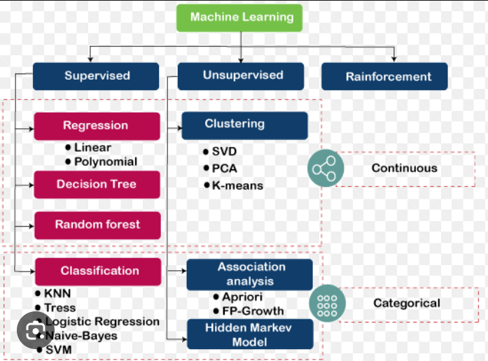

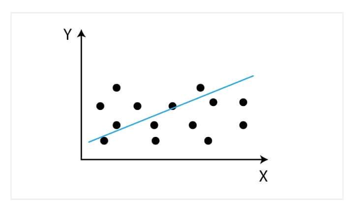
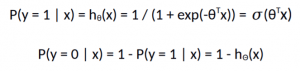
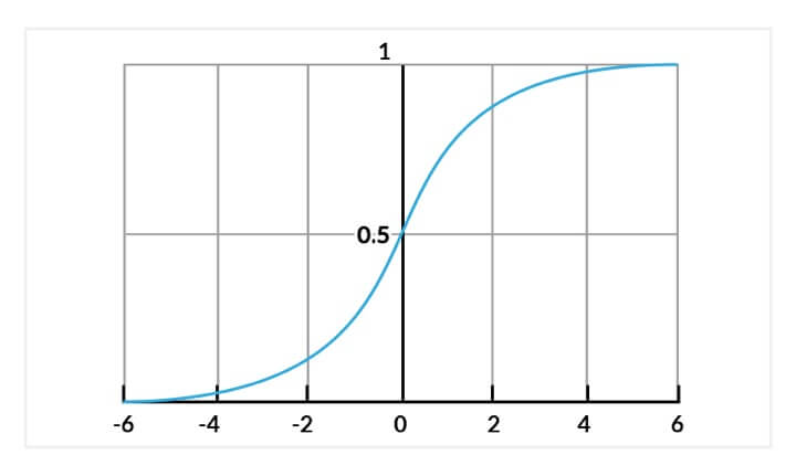
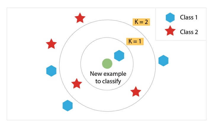
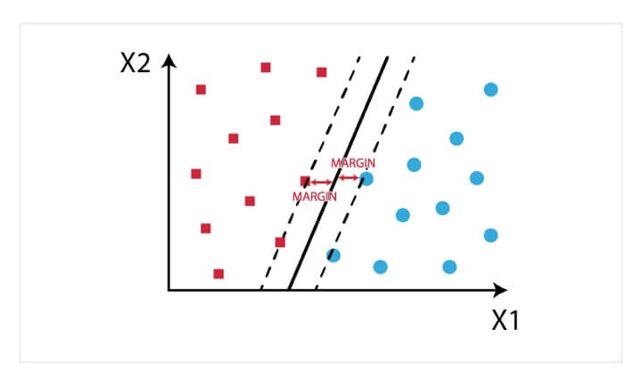
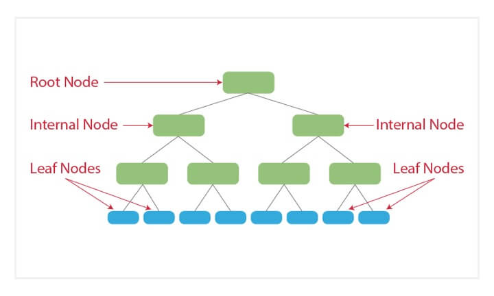
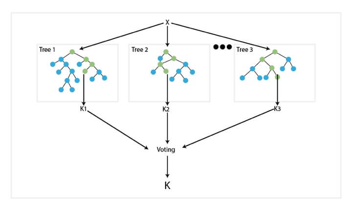
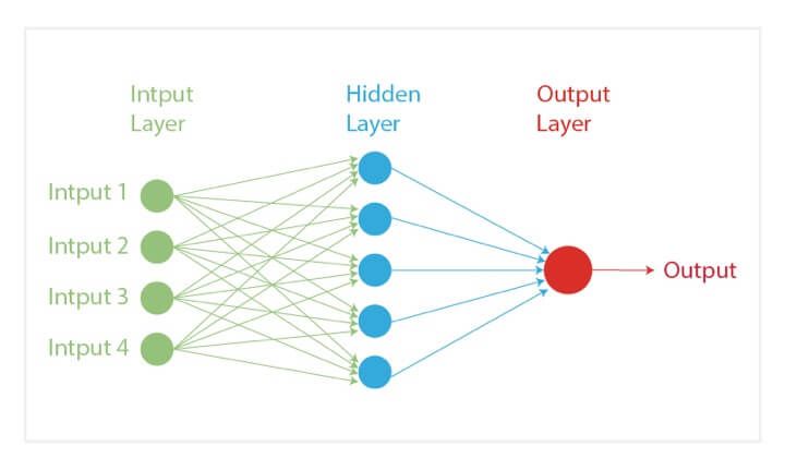
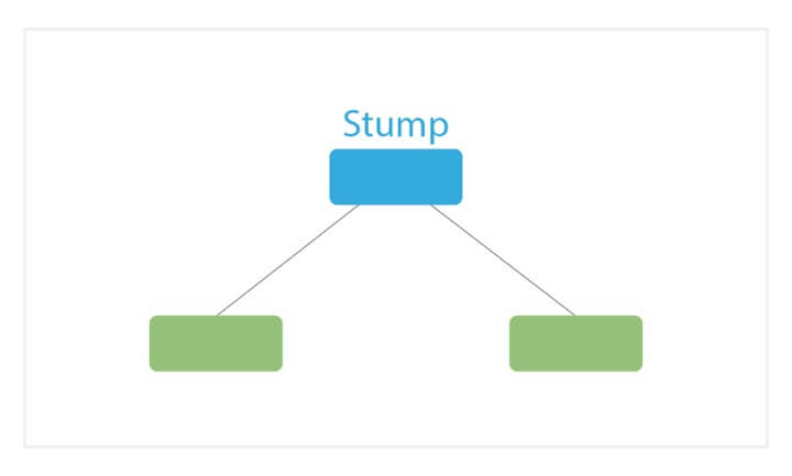
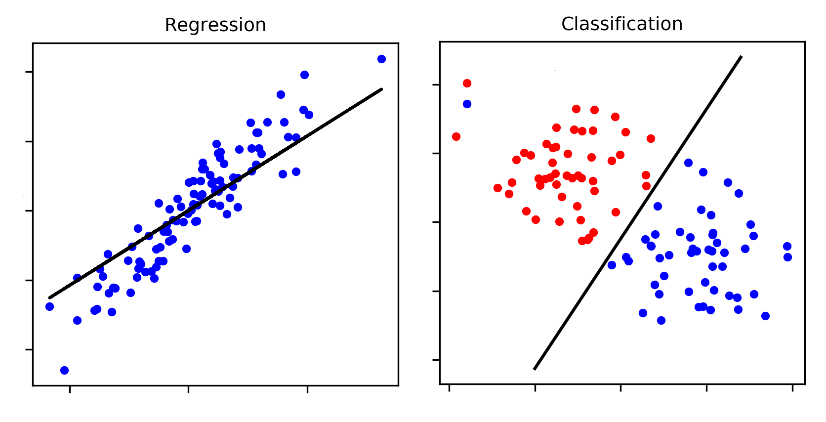
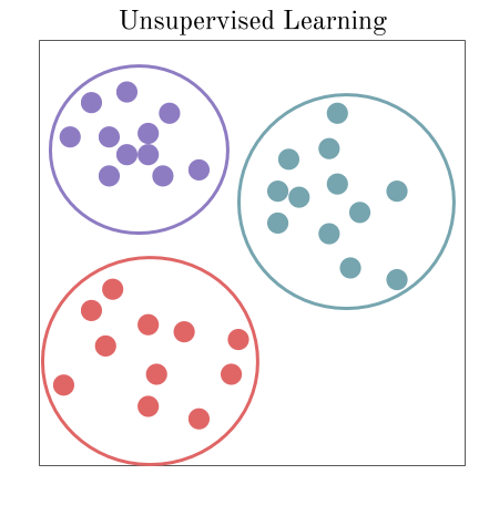
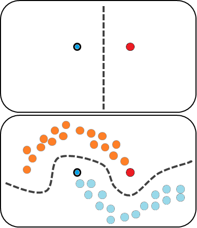

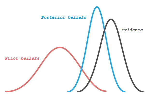
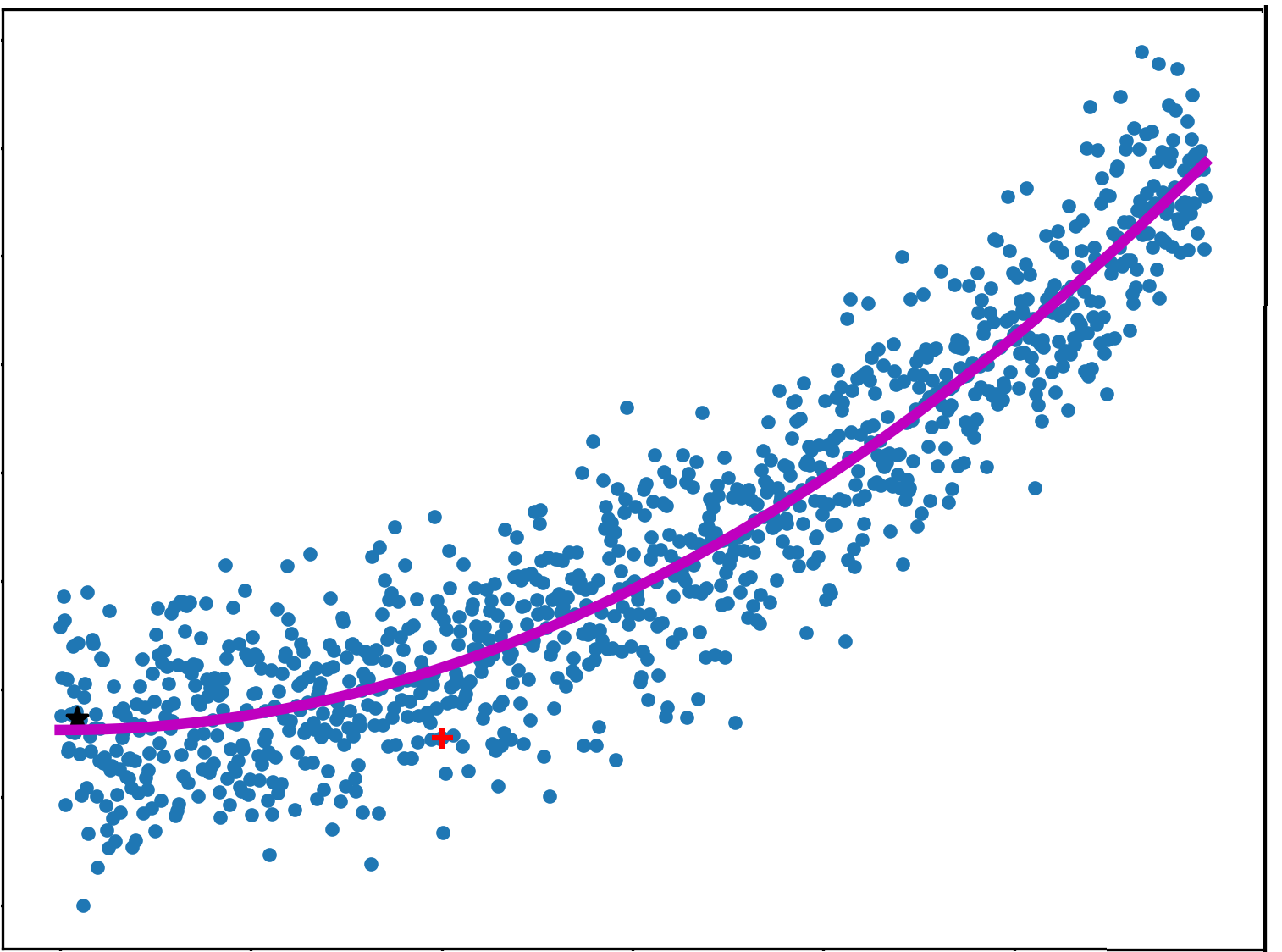

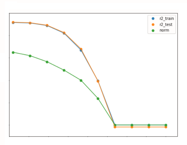
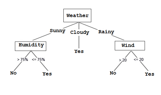
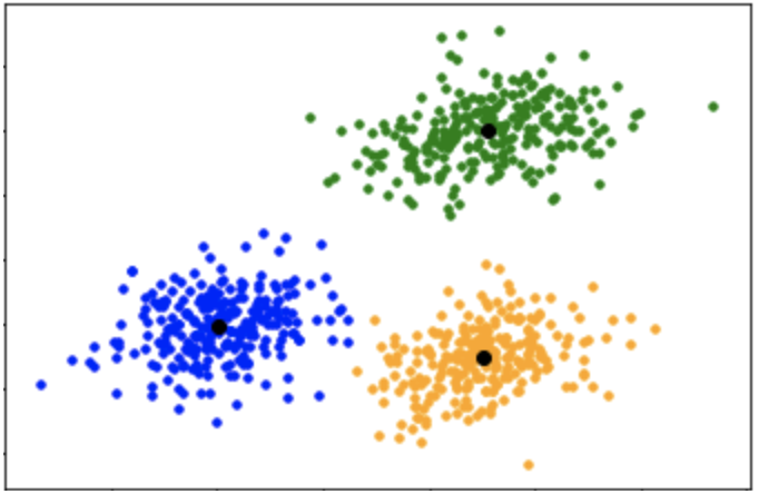
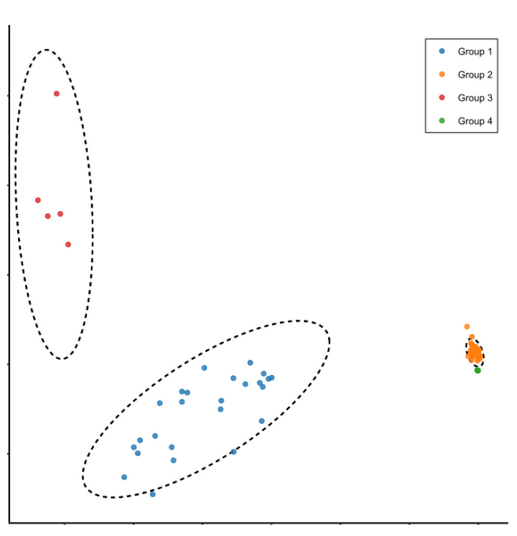
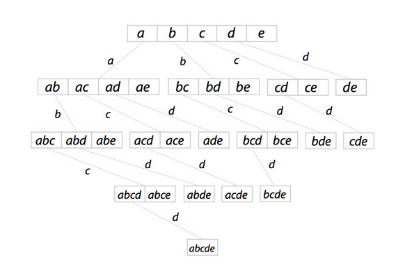
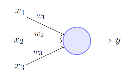
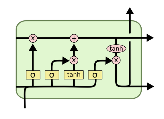
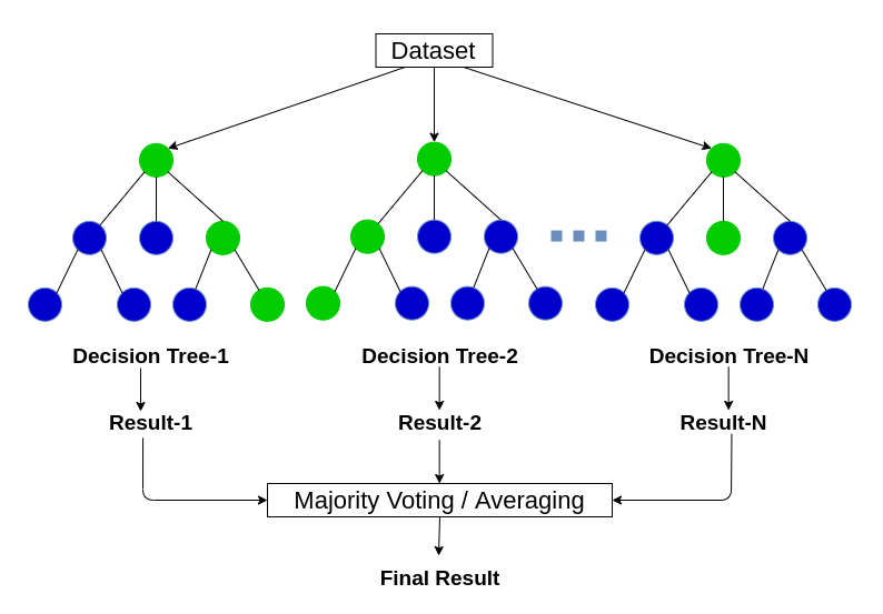
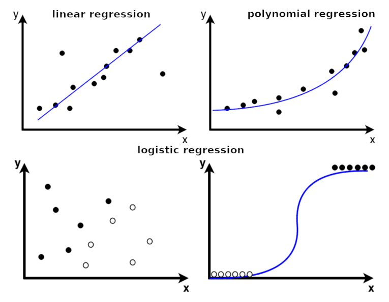
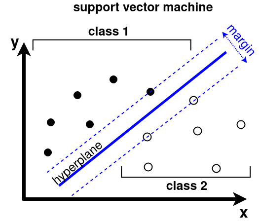

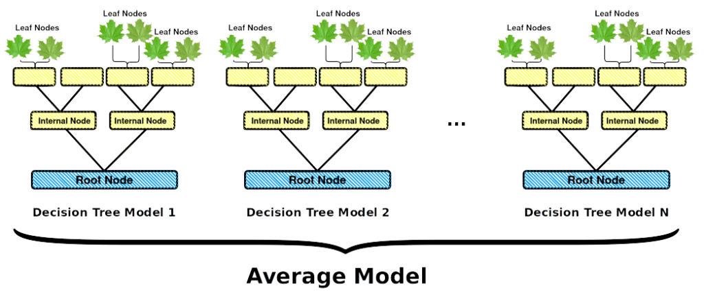
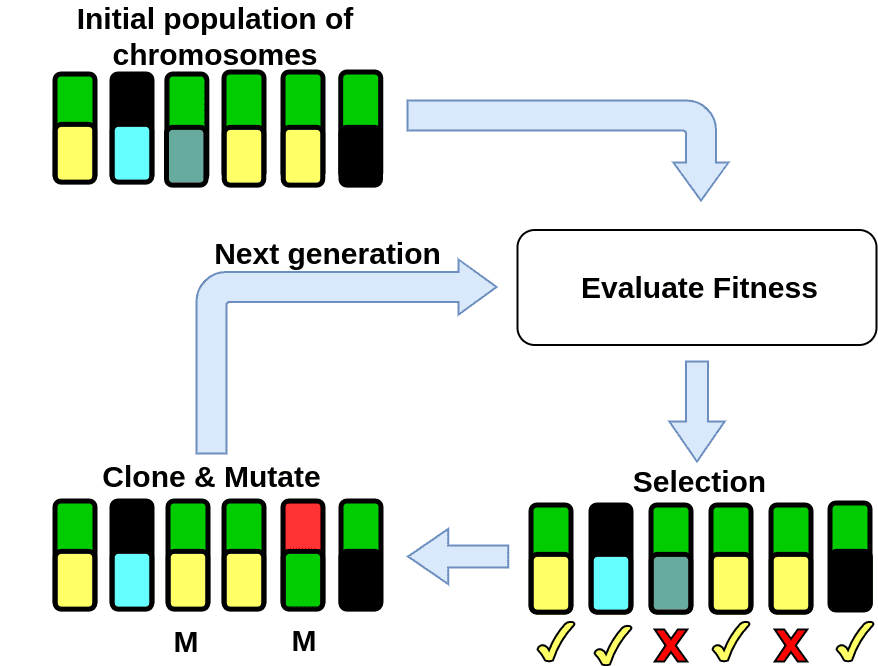
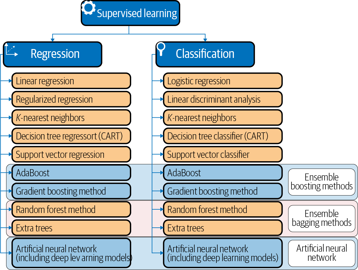
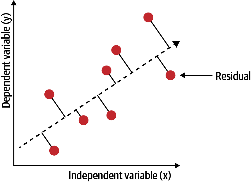
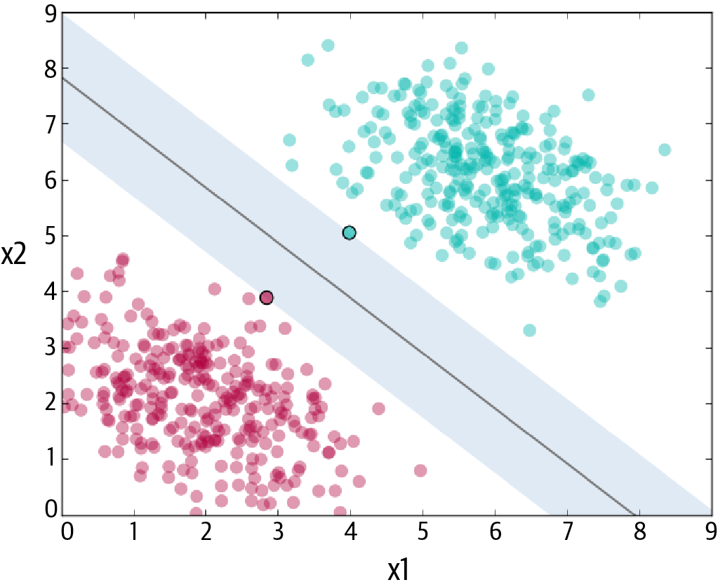
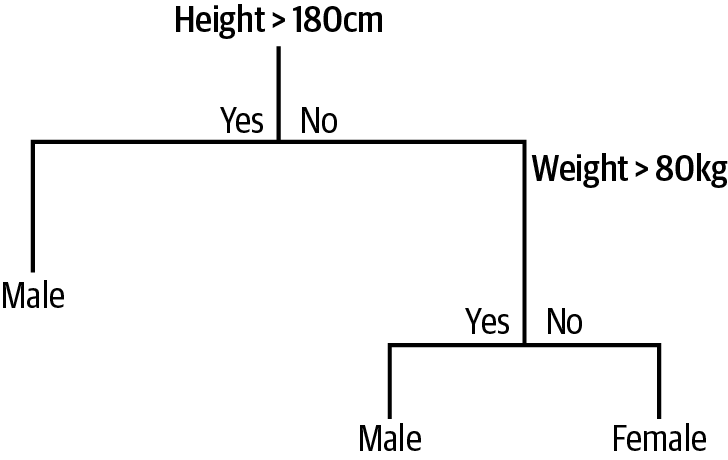
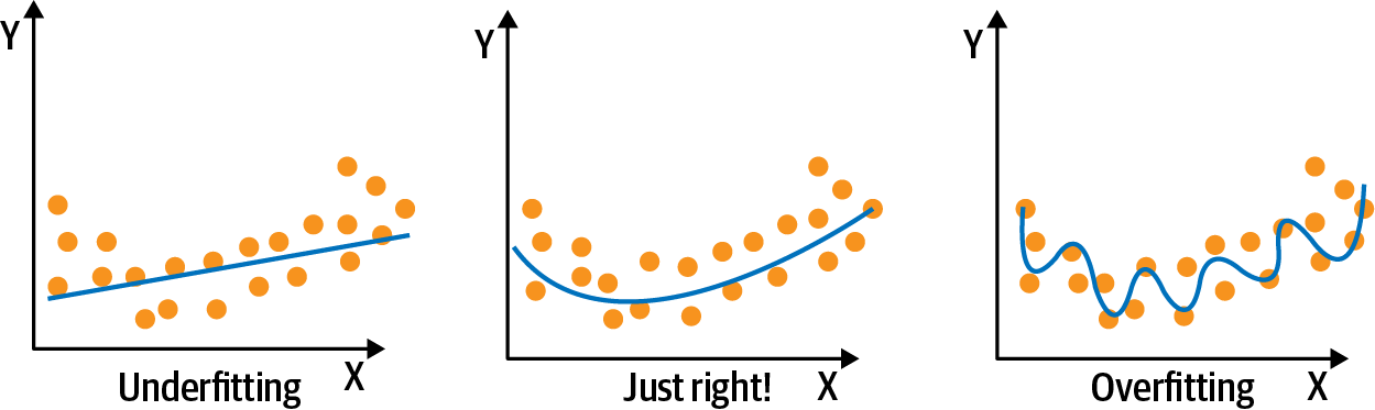
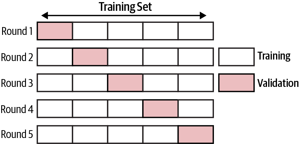
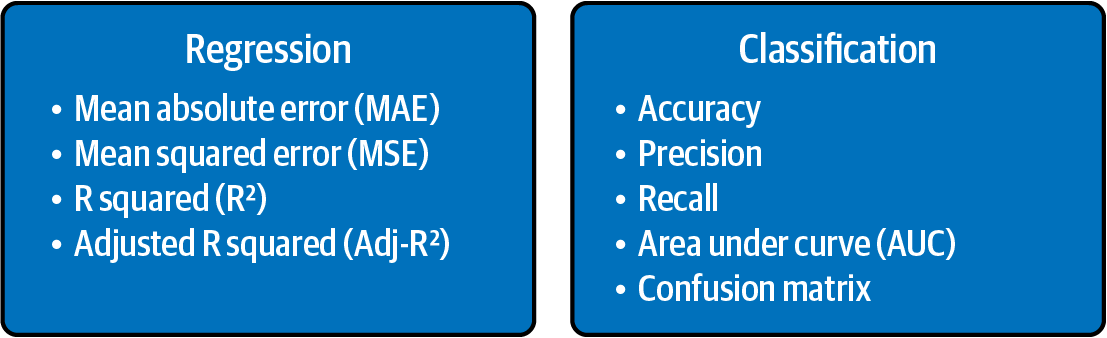
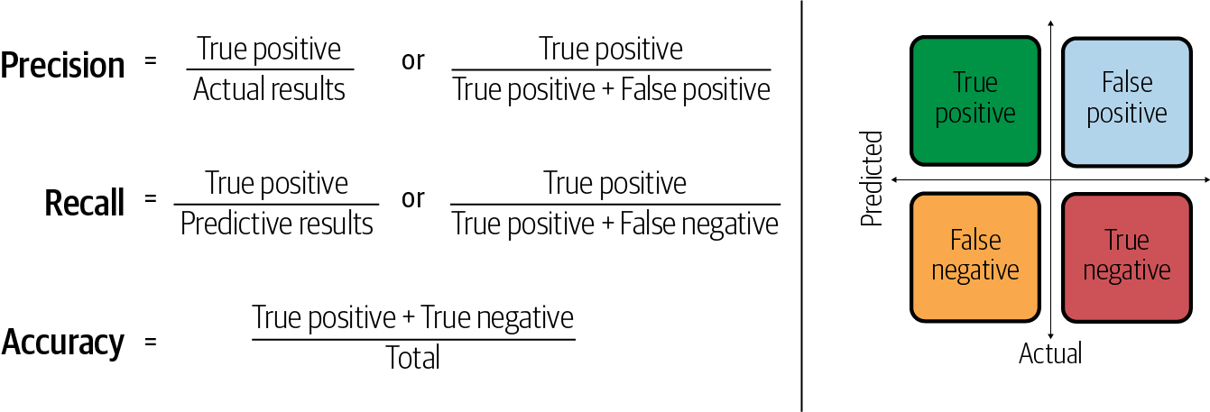
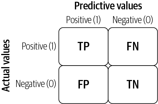
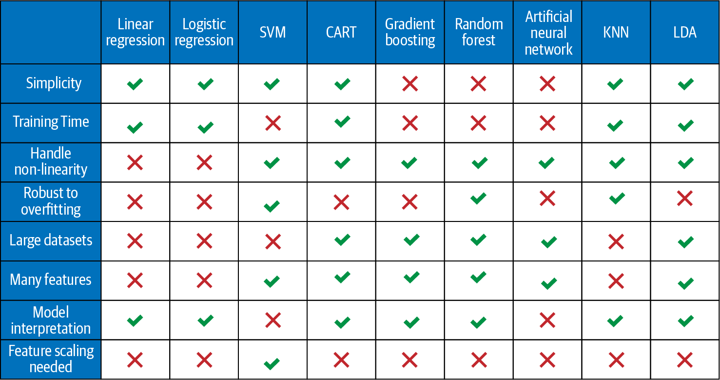

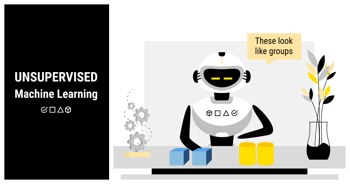
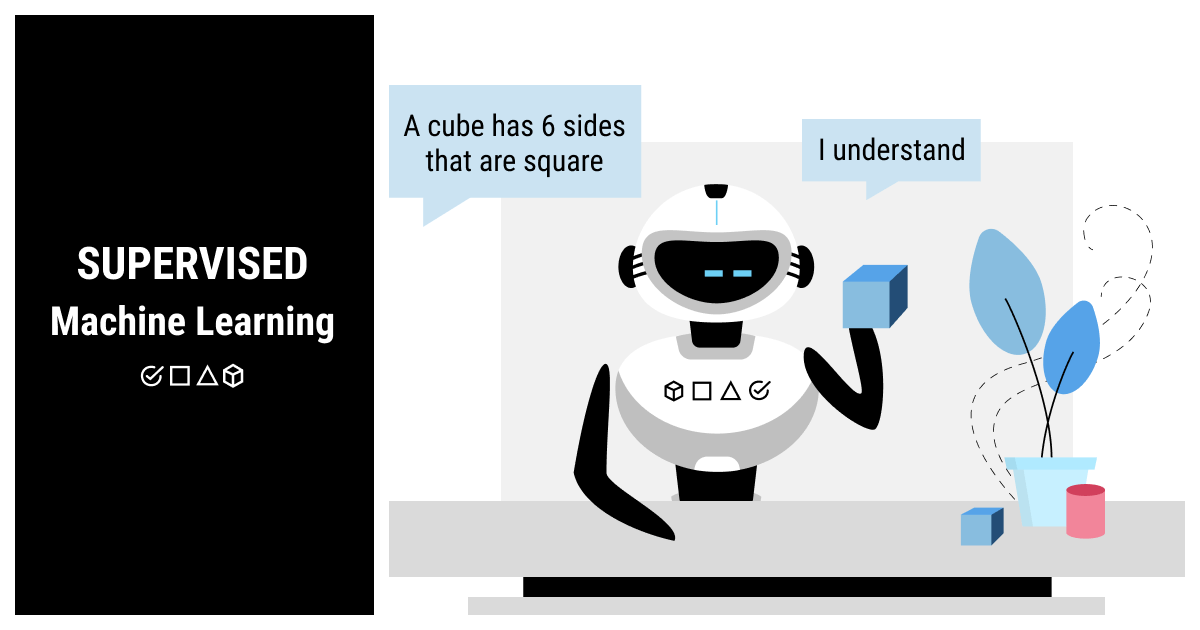
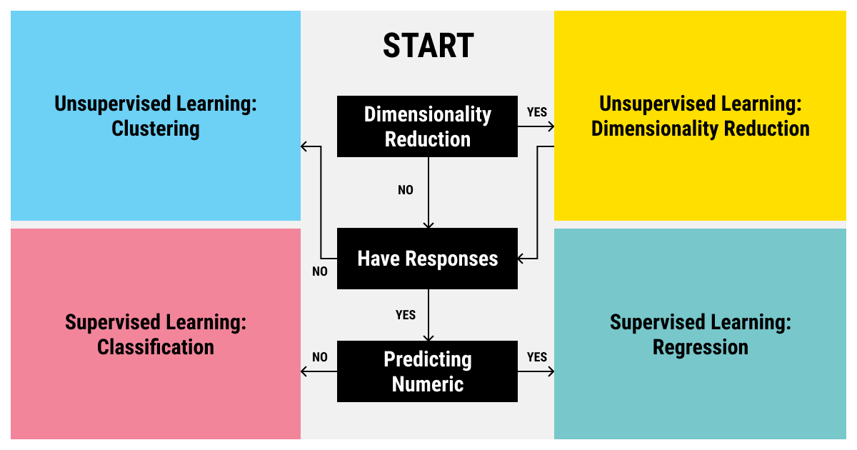
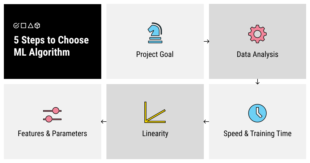
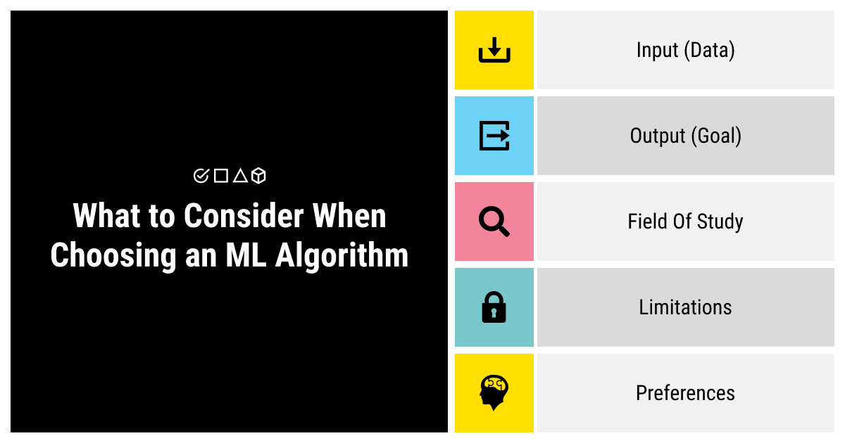


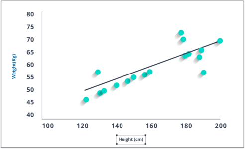
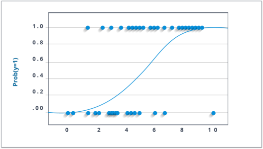
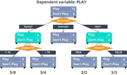

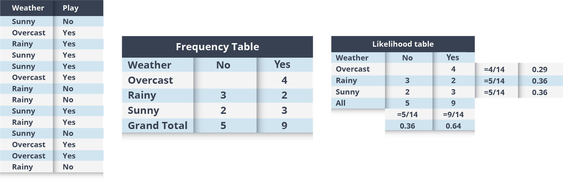

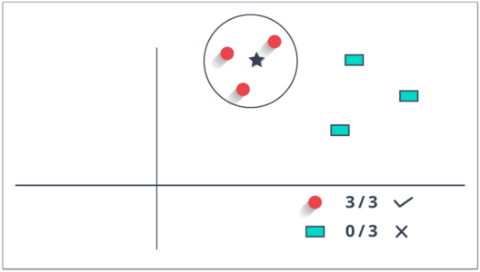
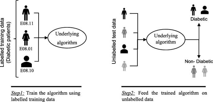
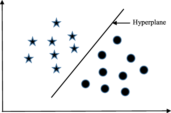
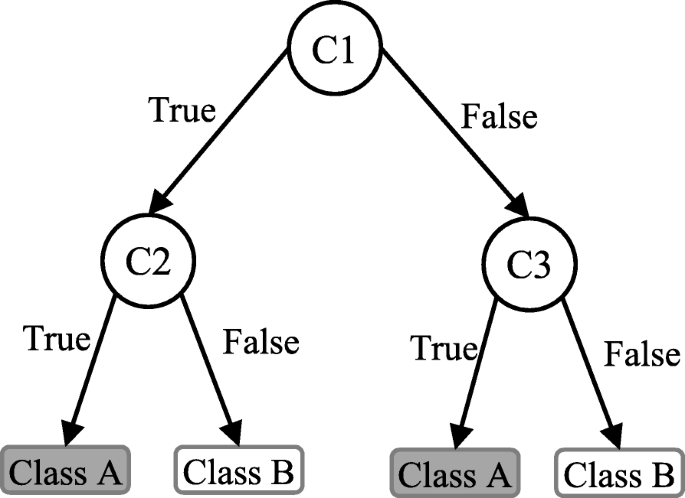
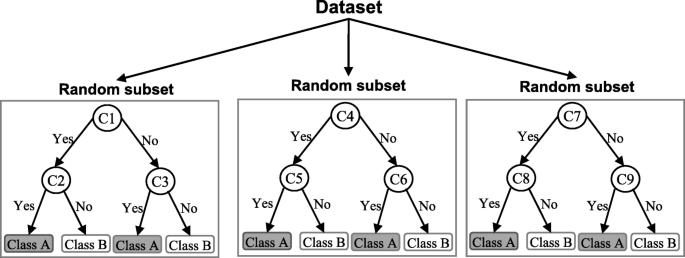
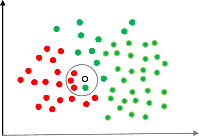
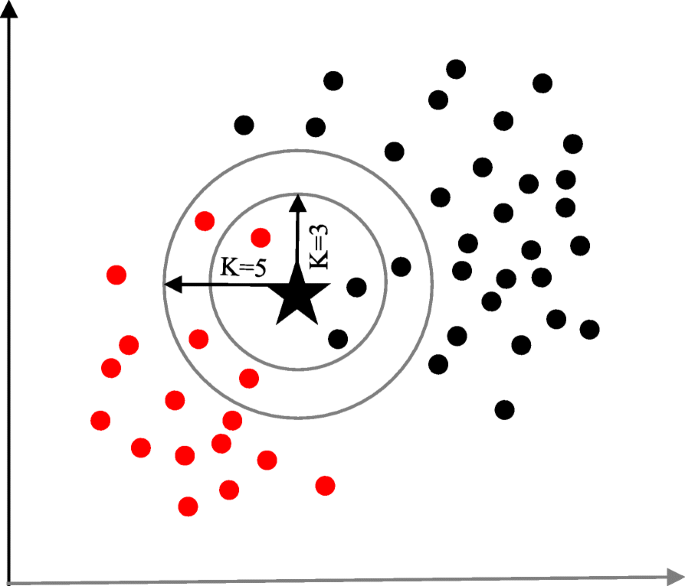
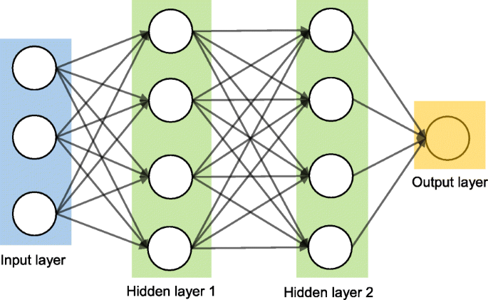
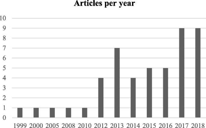
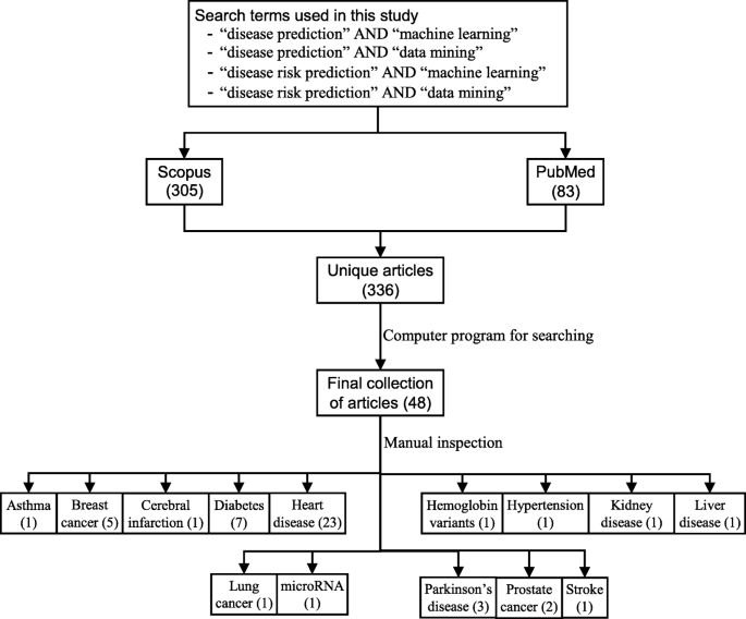
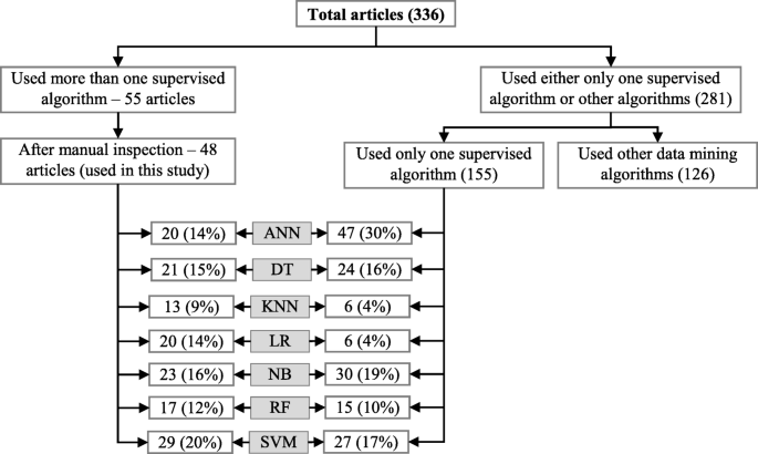
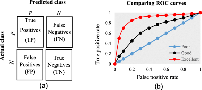
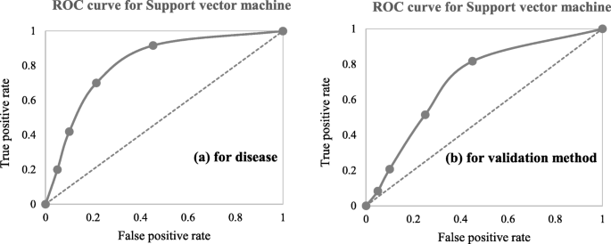
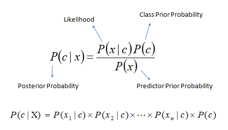