Table of Contents

• Common Machine Learning Algorithms for Beginners in Data Science
  • What are machine learning algorithms?
  • Types of Machine Learning Algorithms
    • 1) Supervised Machine Learning Algorithms
    • 2) Unsupervised Machine Learning Algorithms
    • 3) Reinforcement Machine Learning Algorithms
  • List of Most Used  Popular Machine Learning Algorithms Every Engineer must know
  • Different Machine Learning Algorithms for Beginners
  • Naive Bayes Classifier Algorithm
    • When to use the Naive Bayes Classifier algorithm?
    • Applications of Naive Bayes Classifier
    • Advantages of the Naive Bayes Classifier Algorithm
  • K Means Clustering Algorithm
    • Advantages of using K-Means Clustering
    • Applications of K-Means Clustering
  • Support Vector Machines
    • SVMs are classified into two categories
    • Advantages of Using SVM
    • Applications of Support Vector Machine
  • Apriori Algorithm
    • Principle on which Apriori Algorithm works
    • Advantages of Apriori Algorithm
    • Applications of Apriori Algorithm
  • Linear Regression 
    • Advantages of Linear Regression
    • Applications of Linear Regression
  • Logistic Regression
    • Types of Logistic Regression
    • When to Use Logistic Regression
    • Advantages of Using Logistic Regression
    • Drawbacks of Using Logistic Regression
    • Applications of Logistic Regression
  • Decision Tree 
    • Types of Decision Trees
    • Why should you use the Decision Tree algorithm?
    • When to use Decision Tree 
    • Advantages of Using Decision Tree
    • Drawbacks of Using Decision Tree
    • Applications of Decision Tree 
  • Random Forest
    • Why use Random Forest Algorithm?
    • Advantages of Using Random Forest
    • Drawbacks of Using Random Forest
    • Applications of Random Forest
  • Artificial Neural Networks
    • How do Artificial Neural Network algorithms work?
    • Why use ANNs?
    • Advantages of Using ANNs
    • Disadvantages of Using ANNs
    • Applications of ANNs
  • K-Nearest Neighbors
    • Advantages of Using K-Nearest Neighbors
    • Disadvantages of Using K-Nearest Neighbors
  • Advanced Machine Learning Algorithms Examples
  • Gradient Boosting 
    • XgBoost 
    • CatBoost
    • Light GBM
  • Linear Discriminant Analysis 
    • Advantages of Linear Discriminant Analysis
    • Disadvantages of Linear Discriminant Analysis
    • Applications of Linear Discriminant Analysis
  • Quadratic Discriminant Analysis
    • Advantages of Quadratic Discriminant Analysis
    • Disadvantages of Quadratic Discriminant Analysis
    • Applications of Quadratic Discriminant Analysis
  • Principal Component Analysis 
    • Advantages of Principal Component Analysis
    • Disadvantages of Principal Component Analysis
    • Applications of Principal Component Analysis
  • General Additive Models (GAMs) 
    • Advantages of General Additive Models
    • Disadvantages of General Additive Models
    • Applications of General Additive Models
  • Polynomial Regression
    • Advantages of Polynomial Regression
    • Disadvantages of Polynomial Regression
    • Applications of Polynomial Regression
  • FAQs
    • What are the three types of Machine Learning?
    • Which language is the best for machine learning?
    • What is the simplest machine learning algorithm?
    • What are algorithms in machine learning?
    • Which algorithm is best for machine learning?
    • What are the common machine learning algorithms?

Common Machine Learning Algorithms for Beginners in Data Science

According to a recent study, machine learning algorithms are expected to replace 25% of the jobs across the world in the next ten years. With the rapid growth of big data and the availability of programming tools like Python and R–machine learning (ML) is gaining mainstream presence for data scientists. Machine learning applications are highly automated and self-modifying improving over time with minimal human intervention as they learn with more data. For instance, Netflix’s recommendation algorithm learns more about the likes and dislikes of a viewer based on the shows every viewer watches. Specialized machine learning algorithms have been developed to perfectly address the complex nature of various real-world data problems. For beginners who are struggling to understand the basics of machine learning, here is a brief discussion on the top machine learning algorithms used by data scientists.

What are machine learning algorithms?

A machine learning algorithm can be related to any other algorithm in computer science. An ML algorithm is a procedure that runs on data and is used for building a production-ready machine learning model. If you think of machine learning as the train to accomplish a task, machine learning algorithms will seem like the engines driving its accomplishment. Which type of algorithm in machine learning works best depends on the business problem you are solving, the nature of the dataset, and the resources available.

Types of Machine Learning Algorithms

Machine Learning algorithms are classified as –

1) Supervised Machine Learning Algorithms

Machine learning algorithms that make predictions on a given set of samples. Supervised ML algorithm searches for patterns within the value labels assigned to data points. Some popular machine learning algorithms for Supervised Learning include SVM for classification problems, Linear Regression for regression problems, and Random forest for regression and classification problems. Supervised Learning is when the data set contains annotations with output classes that form the cardinal out classes. E.g., in sentiment analysis, the output classes are happy, sad, angry, etc.

2) Unsupervised Machine Learning Algorithms

There are no labels associated with data points. These machine learning algorithms organize the data into a group of clusters to describe its structure and make complex data look simple and organized for analysis. Unsupervised Learning is where the output variable classes are undefined. The best example of such a classification is clustering. Clustering groups similar objects/data together, thus forming segregated clusters. Clustering also helps in finding biases in the data set. Biases are inherent dependencies in the data set that links the occurrence of values in some way.

Unsupervised Learning is relatively harder, and sometimes the clusters obtained are difficult to understand because of the lack of labels or classes.

3) Reinforcement Machine Learning Algorithms

Reinforcement Learning steers through learning a real-world problem using rewards and punishments are reinforcements. Ideally, a job or activity needs to be discovered or mastered, and the model is rewarded if it completes the job and punished when it fails. The problem with Reinforcement Learning is to figure out what kind of rewards and punishment would be suited for the model.

These algorithms choose an action based on each data point and later learn how good the decision was. Over time, the algorithm changes its strategy to know better and achieve the best reward.

New Projects

COVID-19 Data Analysis Project using Python and AWS StackView Project

Build an ETL Pipeline with Talend for Export of Data from CloudView Project

Build CI/CD Pipeline for Machine Learning Projects using JenkinsView Project

AWS CDK and IoT Core for Migrating IoT-Based Data to AWSView Project

Build a Real-Time Spark Streaming Pipeline on AWS using ScalaView Project

Multilabel Classification Project for Predicting Shipment ModesView Project

A/B Testing Approach for Comparing Performance of ML ModelsView Project

Build an ETL Pipeline on EMR using AWS CDK and Power BIView Project

Migration of MySQL Databases to Cloud AWS using AWS DMSView Project

Multilabel Classification Project for Predicting Shipment ModesView Project

COVID-19 Data Analysis Project using Python and AWS StackView Project

Build an ETL Pipeline with Talend for Export of Data from CloudView Project

Build CI/CD Pipeline for Machine Learning Projects using JenkinsView Project

AWS CDK and IoT Core for Migrating IoT-Based Data to AWSView Project

Build a Real-Time Spark Streaming Pipeline on AWS using ScalaView Project

Multilabel Classification Project for Predicting Shipment ModesView Project

A/B Testing Approach for Comparing Performance of ML ModelsView Project

Build an ETL Pipeline on EMR using AWS CDK and Power BIView Project

Migration of MySQL Databases to Cloud AWS using AWS DMSView Project

Multilabel Classification Project for Predicting Shipment ModesView Project

View all New Projects

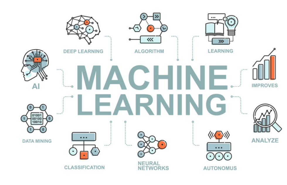
Here is a simple infographic to help you with the best machine learning algorithms examples frequently used by engineers in the artificial intelligence domain.

Different Machine Learning Algorithms for Beginners

Before jumping into the pool of advanced machine learning algorithms, explore these predictive algorithms that will help you master machine learning skills.

Naive Bayes Classifier Algorithm

It would be difficult and practically impossible to manually classify a web page, document, email, or any other lengthy text notes. That is where the Naive Bayes Classifier comes to the rescue. A classifier is a function that allocates a population’s element value from one of the available categories. For instance, Spam Filtering and weather forecast are some popular applications of the Naive Bayes algorithm. The spam filter here is a classifier that assigns a label “Spam” or “Not Spam” to all the emails.

Naïve Bayes Classifier is amongst the most popular learning method grouped by similarities, which works on the famous Bayes Theorem of Probability- to build machine learning models, particularly for disease prediction and document classification. It is a simple classification of words based on the Bayes Probability Theorem for subjective content analysis. This classification method uses probabilities using the Bayes theorem. The basic assumption for the Naive Bayes algorithm is that all the features are considered to be independent of each other. It is a straightforward algorithm, and it is easy to implement. It is beneficial for large datasets and can be implemented for text datasets.

Bayes theorem gives a way to calculate posterior probability P(A|B) from P(A), P(B), and P(B|A).

The formula is given by:  P(A|B) = P(B|A) * P(A) / P(B)

Where P(A|B) is the posterior probability of A given B, P(A) is the prior probability, P(B|A) is the likelihood which is the probability of B given A, and P(B) is the prior probability of B.

When to use the Naive Bayes Classifier algorithm?

1. Naive Bayes is best in cases with a moderate or large training dataset.
2. It works well for dataset instances that have several attributes.
3. Given the classification parameter, attributes that describe the instances should be conditionally independent.

Applications of Naive Bayes Classifier

1. Sentiment Analysis- It is used by Facebook to analyze status updates expressing positive or negative emotions.
2. Document Categorization- Google uses document classification to index documents and finds relevancy scores, i.e., the PageRank. PageRank mechanism considers the pages marked as important in the databases parsed and classified using a document classification technique.
3. This algorithm is also used for classifying news articles about Technology, Entertainment, Sports, Politics, etc.
4. Email Spam Filtering- Google Mail uses the Naive Bayes algorithm to classify your emails as Spam or Not Spam.
5. Data Science Libraries in Python to implement Naive Bayes – Sci-Kit Learn

Advantages of the Naive Bayes Classifier Algorithm

1. The Naive Bayes Classifier algorithm performs well when the input variables are categorical.
2. A Naïve Bayes classifier converges faster, requiring relatively little training data set than other discriminative models like logistic regression when the Naïve Bayes conditional independence assumption holds.
3. With the Naive Bayes Classifier algorithm, predicting the class of the testing data set is more effortless. A good bet for multi-class predictions as well.
4. Though it requires conditional independence assumption, Naïve Bayes Classifier has performed well in various application domains.

K Means Clustering Algorithm

K-means is a popularly used unsupervised ML algorithm for cluster analysis. K-Means is a non-deterministic and iterative method. The algorithm operates on a given data set through a pre-defined number of clusters, k. The output of the K Means algorithm is k clusters with input data partitioned among the clusters. For instance, let’s consider K-Means Clustering for Wikipedia Search results. The search term “Jaguar” on Wikipedia will return all pages containing the word Jaguar which can refer to Jaguar as a Car, Jaguar as Mac OS version, and Jaguar as an Animal. K Means clustering algorithm can be applied to group the web pages that talk about similar concepts. So, the algorithm will group all the web pages that refer to Jaguar as an Animal into one cluster, Jaguar as a Car into another cluster, and so on.

For any new incoming data point, the data point is classified according to its proximity to the nearby classes. Datapoints inside a cluster will exhibit similar characteristics while the other clusters will have different properties. The primary example of clustering would be grouping the same customers in a particular class for any marketing campaign, and it is also a practical algorithm for document clustering. 

The steps followed in the k means algorithm are as follows – 

1. Specify the number of clusters as k
2. Randomly select k data points and assign them to the clusters
3. Cluster centroids will be calculated subsequently
4. Keep iterating from 1-3 steps until you find the optimal centroid, after which values won’t change. 

i) The sum of the squared distance between the centroid and the data point is computed.

ii) Assign each data point to the cluster that is closer to the other cluster

iii) Compute the centroid for the cluster by taking the average of all the data points in the cluster

We can find the optimal number of clusters k by plotting the value of the sum squared distance which decreases gradually to reach an optimal number of k. 

Advantages of using K-Means Clustering

1. In the case of globular clusters, K-Means produce tighter clusters than hierarchical clustering.
2. Given a smaller value of K, K-Means clustering computes faster than hierarchical clustering for many variables.

Applications of K-Means Clustering

Most search engines like Yahoo and Google use the K Means Clustering algorithm to cluster web pages by similarity and identify the ‘relevance rate’ of search results. This helps search engines reduce the computational time for the users.

Data Science Libraries in Python to implement K-Means Clustering – SciPy, Sci-Kit Learn, Python Wrapper

Data Science Libraries in R to implement K-Means Clustering – stats.

Support Vector Machines

Support Vector Machine is a supervised learning algorithm for classification or regression problems where the dataset teaches SVM about the classes so that SVM can classify any new data. It organizes the data into different categories by finding a line (hyperplane) separating the training data set into classes. As there are many such linear hyperplanes, the SVM algorithm tries to maximize the distance between the various classes involved, referred to as margin maximization. If the line that maximizes the distance between the classes is identified, the probability of generalizing well to unseen data is increased.

SVMs are classified into two categories

1. Linear SVMs – In linear SVMs, the training data i.e. classifiers, are separated by a hyperplane.
2. Non-Linear SVMs- In non-linear SVMs, it is impossible to separate the training data using a hyperplane. For example, the training data for Face detection consists of a group of images that are faces and another group of images that do not face (in other words, all other images in the world except faces). Under such conditions, the training data is too complex that it is impossible to find a representation for every feature vector. Separating the set of faces linearly from the set of non-face is a complicated task.

Advantages of Using SVM

1. SVM offers the best classification performance (accuracy) on the training dataset.
2. SVM renders more efficiency for the correct classification of future data.
3. The best thing about SVM is that it does not make strong assumptions about data.
4. It does not overfit the data.

Applications of Support Vector Machine

SVM is commonly used for stock market forecasting by various financial institutions. For instance, one can use it to compare the relative performance of the stocks to those of other stocks in the same sector. The close comparison of stocks helps manage investment-making decisions based on the classifications made by the SVM learning algorithm.

Explore Enterpirse-Grade Data Science Projects for Resume Building and Ace your Next Job Interview!

Apriori Algorithm

Apriori algorithm is an unsupervised ML algorithm that generates association rules from a given data set. The Association rule implies that if item A occurs, then item B also occurs with a certain probability. Most of the association rules generated are in the IF_THEN format. For example, IF people buy an iPad, they also buy an iPad Case to protect it. For the algorithm to derive such conclusions, it first observes the number of people who bought an iPad case while purchasing an iPad. This way a ratio is derived like out of the 100 people who purchased an iPad, 85 people also purchased an iPad case.

Principle on which Apriori Algorithm works

1. If an item set frequently occurs, then all the subsets of the item set also happen often.
2. If an item set occurs infrequently, then all the supersets of the item set have infrequent occurrences.

Advantages of Apriori Algorithm

1. It is easy to implement and can be parallelized easily.
2. Apriori implementation makes use of large item set properties.

Applications of Apriori Algorithm

1. Detecting Adverse Drug Reactions – Apriori algorithm is used for association analysis on healthcare data like the drugs taken by patients, characteristics of each patient, adverse ill-effects patients experience, initial diagnosis, etc. This analysis produces association rules that help identify the combination of patient characteristics and medications that lead to adverse side effects of the drugs
2. Market Basket Analysis – Many e-commerce giants like Amazon use Apriori to draw data on which products are likely to be purchased together and which are most responsive to promotion. For example, a retailer might use Apriori to predict that people who buy sugar and flour will likely buy eggs to bake a cake
3. Auto-Complete Applications – Google auto-complete is another popular application of Apriori wherein – when the user types a word, the search engine looks for other associated words that people usually type after a specific word.

Data Science Libraries in Python to implement Apriori Algorithm – There is a python implementation for Apriori in PyPi

Data Science Libraries in R to implement Apriori Algorithm – arules

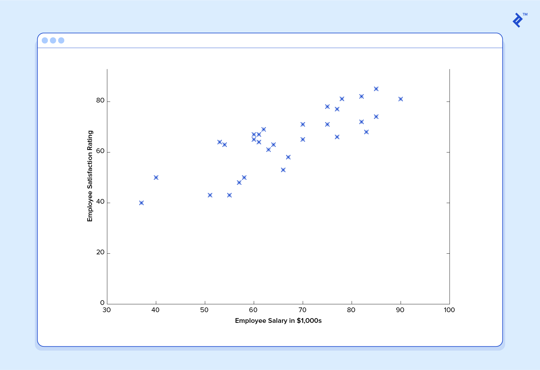
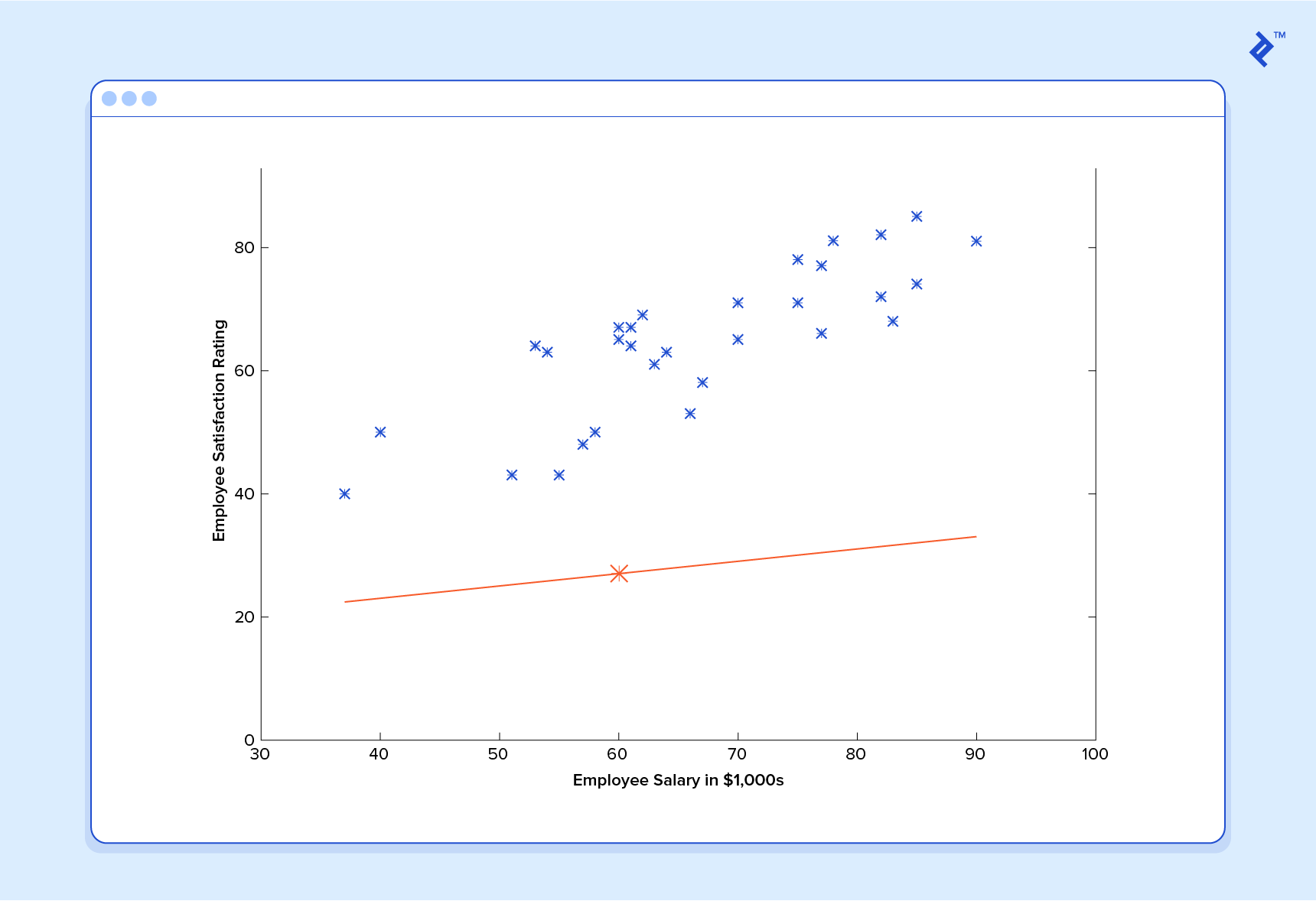
Linear Regression 

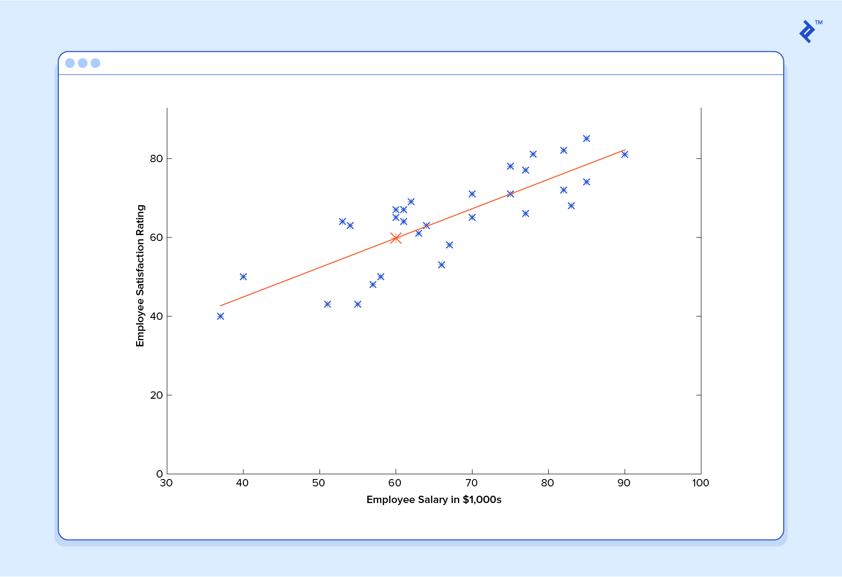
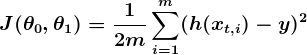
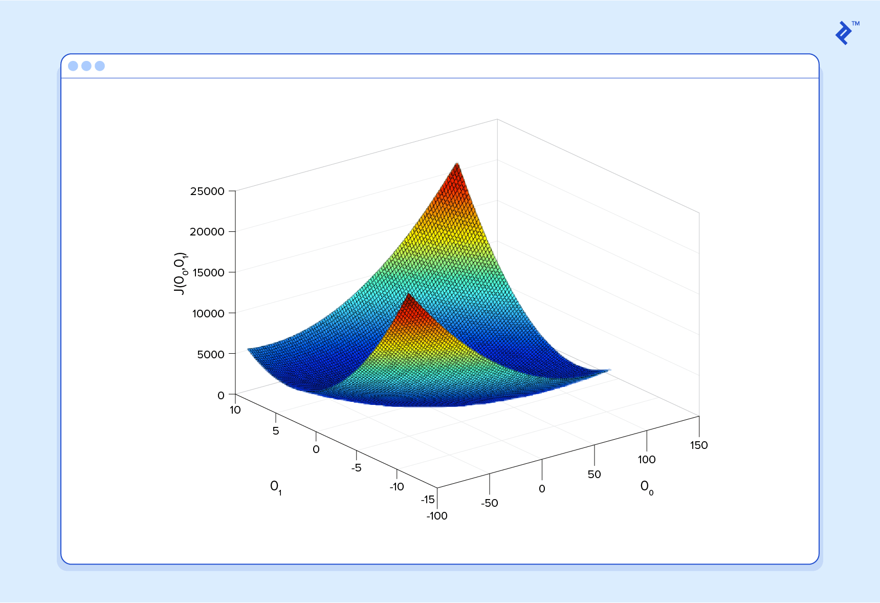
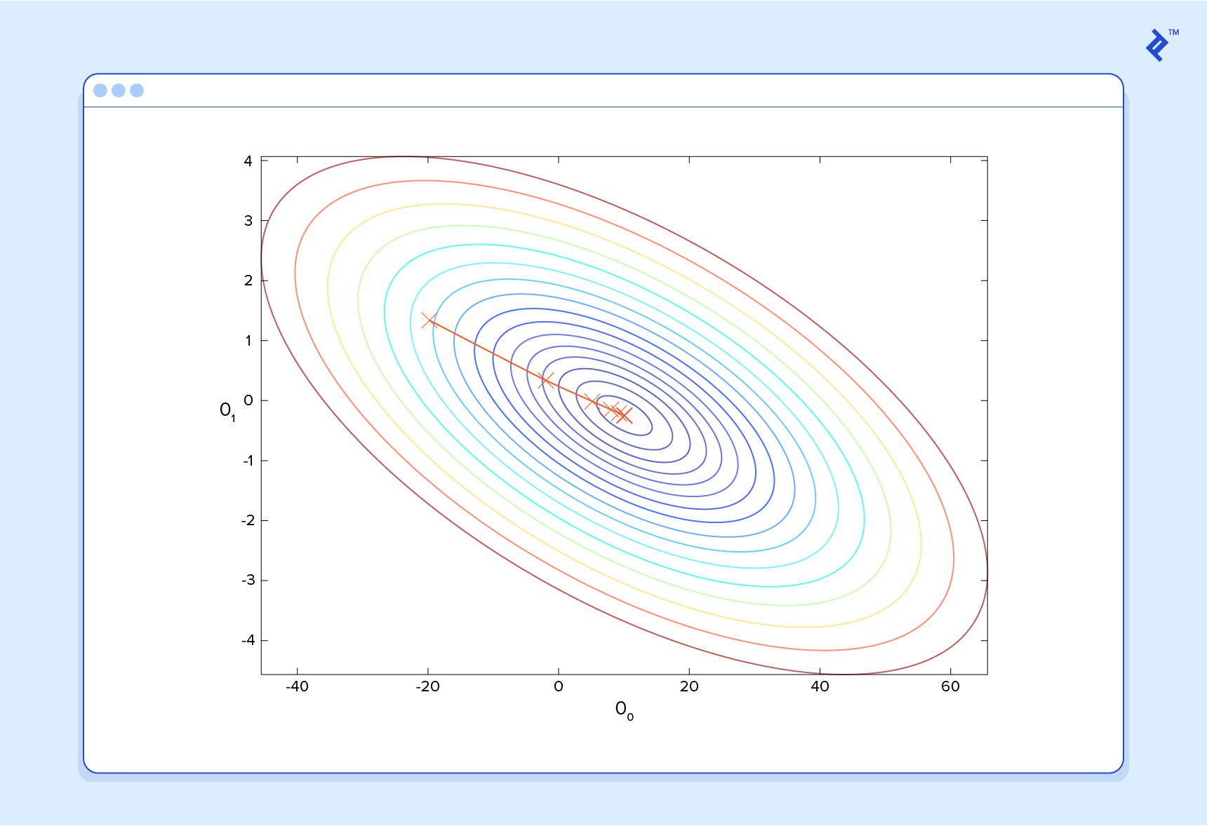
The linear Regression model shows the relationship between 2 variables and how the change in one variable impacts the other. The algorithm shows the impact of the dependent variable on changing the independent variable. The independent variables are referred to as explanatory variables, which explain the factors that impact the dependent variable. The dependent variable is often referred to as the factor of interest or predictor. The linear regression model is used for estimating fundamental continuous values. The most common linear regression examples are housing price predictions, sales predictions, weather predictions, employee salary estimations, etc. The primary goal for linear regression is to fit the best line amongst the predictions. The equation for simple linear regression is Y=a*x+b, where y is the dependent variable, x is the set of independent variables, a is the slope, and b is the intercept. 

The best example from human lives would be how a child would solve a simple problem like – ordering the children in class height orderwise without asking the children’s heights. The child will be able to solve this problem by visually looking at the heights of the children and subsequently arranging them height-wise. That is how you can perceive linear regression in a real-life scenario. The weights, which are the heights and the build of the children, have been learned by the child gradually. Looking back at the equation, a and b are the coefficients learned through the regression model by minimizing the sum of squared errors in the model values. 

The graph below shows the relation between the number of umbrellas sold and the rainfall in a particular region –

Advantages of Linear Regression

1. It is one of the most interpretable machine learning algorithms, making it easy to explain to others.
2. It is easy to use as it requires minimal tuning.
3. It is the most widely used machine learning technique that runs fast.

Applications of Linear Regression

1. Estimating Sales
   Linear Regression finds excellent use in business for sales forecasting based on trends. If a company observes a steady increase in sales every month – linear regression analysis of the monthly sales data helps the company forecast sales in upcoming months.
2. Risk Assessment
   Linear Regression helps assess the risk involved in the insurance or financial domain. A health insurance company can do a linear regression analysis on the number of claims per customer against age. This analysis helps insurance companies find that older customers tend to make more insurance claims. Such analysis results play a vital role in critical business decisions and are made to account for risk.

Data Science Libraries in Python to implement Linear Regression – stats model and SciKit

Data Science Libraries in R to implement Linear Regression – stats

Explanations about the top machine learning algorithms will continue, as it is a work in progress. Stay tuned to our blog to learn more about the popular machine learning algorithms and their applications!!!

Logistic Regression

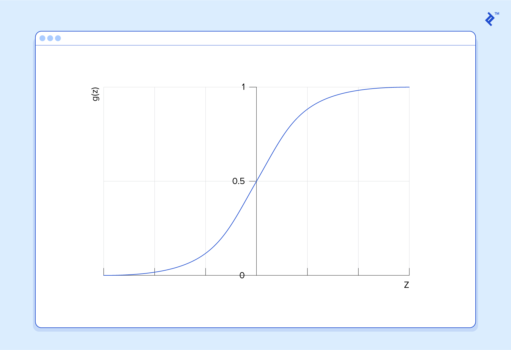
The name of this algorithm could be a little confusing in the sense that this algorithm is used to estimate discrete values in classification tasks and not regression problems. The name ‘Regression’ here implies that a linear model is fit into the feature space. This algorithm applies a logistic function to a linear combination of features to predict the outcome of a categorical dependent variable based on predictor variables. The odds or probabilities that describe the result of a single trial are modeled as a function of explanatory variables. This algorithm helps estimate the likelihood of falling into a specific level of the categorical dependent variable based on the given predictor variables.

Suppose you want to predict if there will be a snowfall tomorrow in New York. Here the prediction outcome is not a continuous number because there will either be snowfall or no snowfall, so simple linear regression cannot be applied. Here the outcome variable is one of the several categories, and logistic regression helps.

Types of Logistic Regression

1. Binary Logistic Regression – The most commonly used logistic regression is when the categorical response has two possible outcomes, i.e., yes or not. Example –Predict whether a student will pass or fail an exam, whether a student will have low or high blood pressure, and whether a tumor is cancerous.
2. Multi-nominal Logistic Regression – Categorical response has three or more possible outcomes with no order. Example- Predicting what kind of search engine (Yahoo, Bing, Google, and MSN) is used by majority of US citizens.
3. Ordinal Logistic Regression – Categorical response has 3 or more possible outcomes with natural ordering. Example- How a customer rates the service and quality of food at a restaurant based on a scale of 1 to 10.

Let us consider a simple example where a cake manufacturer wants to find out if baking a cake at 160°C, 180°C and 200°C will produce a ‘hard’ or ‘soft’ variety of cake ( assuming the fact that the bakery sells both the varieties of cake with different names and prices). Logistic regression is a perfect fit in this scenario instead of other statistical techniques. For example, if the manufacturers produce 2 cake batches wherein the first batch contains 20 cakes (of which 7 were hard and 13 were soft ) and the second batch of cake produced consisted of 80 cakes (of which 41 were hard and 39 were soft cakes). Here in this case if a linear regression algorithm is used it will give equal importance to both the batches of cakes regardless of the number of cakes in each batch. Applying a logistic regression algorithm will consider this factor and give the second batch of cakes more weightage than the first batch.

When to Use Logistic Regression

1. Use logistic regression algorithms when there is a requirement to model the probabilities of the response variable as a function of some other explanatory variable. For example, the probability of buying a product X as a function of gender
2. Use logistic regression algorithms when there is a need to predict probabilities that categorical dependent variables will fall into two categories of the binary response as a function of some explanatory variables. For example, what is the probability that a customer will buy a perfume given that the customer is a female?
3. Logistic regression algorithms is also best suited when the need is to classify elements into two categories based on the explanatory variable. For example-classify females into ‘young’ or ‘old’ group based on their age.

Advantages of Using Logistic Regression

1. Easier to inspect and less complex.
2. Robust algorithm as the independent variables need not have equal variance or normal distribution.
3. These algorithms do not assume a linear relationship between the dependent and independent variables and hence can also handle non-linear effects.
4. Controls confounding and tests interaction.
5. It is one the best machine learning approaches for solving binary classification problems.

Drawbacks of Using Logistic Regression

1. When the training dataset is sparse and high dimensional, in such situations a logistic model may overfit the training dataset.
2. This algorithm cannot predict continuous outcomes. For instance, it cannot be applied when the goal is to determine how heavily it will rain because the scale of measuring rainfall is continuous. Data scientists can predict heavy or low rainfall but this would make some compromises with the precision of the dataset.
3. This algorithm requires more data to achieve stability and meaningful results. These algorithms require a minimum of 50 data points per predictor to achieve stable outcomes.
4. It predicts outcomes depending on a group of independent variables and if a data scientist or a machine learning expert goes wrong in identifying the independent variables then the developed model will have minimal or no predictive value.
5. It is not robust to outliers and missing values.

Applications of Logistic Regression

1. This algorithm is applied in the field of epidemiology to identify risk factors for diseases and plan accordingly for preventive measures.
2. It is used to predict whether a candidate will win or lose a political election or whether a voter will vote for a particular candidate.
3. It is used to classify a set of words as nouns, pronouns, verbs, adjectives.
4. It is used in weather forecasting to predict the probability of rain.
5. It is used in credit scoring systems for risk management to predict the defaulting of an account.

The Data Science libraries in Python language to implement Logistic Regression Algorithm is Sci-Kit Learn.

The Data Science libraries in R language to implement Logistic Regression Algorithm is stats package (glm () function)  

Decision Tree 

You are making a weekend plan to visit the best restaurant in town as your parents are visiting but you are hesitant in making a decision on which restaurant to choose. Whenever you want to visit a restaurant you ask your friend Tyrion if he thinks you will like a particular place. To answer your question, Tyrion first has to find out the kind of restaurants you like. You give him a list of restaurants that you have visited and tell him whether you liked each restaurant or not (giving a labeled training dataset). When you ask Tyrion that whether you will like a particular restaurant R or not, he asks you various questions like “Is “R” a rooftop restaurant?” , “Does restaurant “R” serve Italian cuisine?”, “Does R have live music?”, “Is restaurant R open till midnight?” and so on. Tyrion asks you several informative questions to maximize the information gain and gives you YES or NO answer based on your answers to the questionnaire. Here Tyrion is a decision tree for your favourite restaurant preferences.

A decision tree is a graphical representation that makes use of branching methodology to exemplify all possible outcomes of a decision, based on certain conditions. In a decision tree, the internal node represents a test on the attribute, each branch of the tree represents the outcome of the test and the leaf node represents a particular class label i.e. the decision made after computing all of the attributes. The classification rules are represented through the path from root to the leaf node.

---

---

Types of Decision Trees

Classification Trees- These are considered as the default kind of decision trees used to separate a dataset into different classes, based on the response variable. These are one of the highly sophisticated classification methods for cases where the response variable is categorical in nature.

Regression Trees-When the response or target variable is continuous or numerical, regression trees are used.

Decision trees can also be classified into two types, based on the type of target variable- Continuous Variable Decision Trees and Binary Variable Decision Trees. It is the target variable that helps decide what kind of decision tree would be required for a particular problem.

Why should you use the Decision Tree algorithm?

1. These machine learning algorithms help make decisions under uncertainty and help you improve communication, as they present a visual representation of a decision situation.
2. Decision tree helps a data scientist capture the idea that if a different decision was taken, then how the operational nature of a situation or model would have changed intensely.
3. Decision tree algorithms help make optimal decisions by allowing a data scientist to traverse through forward and backward calculation paths.

When to use Decision Tree 

1. Decision trees are robust to errors and if, the training dataset contains errors- decision tree algorithms will be best suited to address such problems.
2. They are best suited for problems where instances are represented by attribute value pairs.
3. If the training dataset has missing value then decision trees can be used, as they can handle missing values nicely by looking at the data in other columns.
4. They are best suited when the target function has discrete output values.

Advantages of Using Decision Tree

1. Decision trees are very instinctual and can be explained to anyone with ease. People from a non-technical background can also decipher the hypothesis drawn from a decision tree, as they are self-explanatory.
2. When using this algorithm, data type is not a constraint as they can handle both categorical and numerical variables.
3. Decision tree machine learning algorithms do not require making any assumption on the linearity in the data and hence can be used in circumstances where the parameters are non-linearly related. These machine learning algorithms do not make any assumptions on the classifier structure and space distribution.
4. These algorithms are useful in data exploration. Decision trees implicitly perform feature selection which is very important in predictive analytics. When a decision tree is fit to a training dataset, the nodes at the top on which the tree is split, are considered as important variables within a given dataset and feature selection is completed by default.
5. Decision trees help save data preparation time, as they are not sensitive to missing values and outliers. Missing values will not stop you from splitting the data for building a decision tree. Outliers will also not affect the decision trees as data splitting happens based on some samples within the split range and not on exact absolute values.

Drawbacks of Using Decision Tree

1. The more the number of decisions in a tree, less is the accuracy of any expected outcome.
2. A major drawback of this machine learning algorithm is that the outcomes may be based on expectations. When decisions are made in real-time, the payoffs and resulting outcomes might not be the same as expected or planned. There are chances that this could lead to unrealistic decision trees leading to bad decision making. Any irrational expectations could lead to major errors and flaws in decision tree analysis, as it is not always possible to plan for all eventualities that can arise from a decision.
3. Decision Trees do not fit well for continuous variables and result in instability and classification plateaus.
4. Decision trees are easy to use when compared to other decision making models but creating large decision trees that contain several branches is a complex and time consuming task.
5. Decision tree considers only one attribute at a time and might not be best suited for actual data in the decision space.
6. Large sized decision trees with multiple branches are not comprehensible and pose several presentation difficulties.

Applications of Decision Tree 

1. Decision trees are among the popular machine learning algorithms that find great use in finance for option pricing.
2. Remote sensing is an application area for pattern recognition based on decision trees.
3. Decision tree algorithms are used by banks to classify loan applicants by their probability of defaulting payments.
4. Gerber Products, a popular baby product company, used decision tree algorithm to decide whether they should continue using the plastic PVC (Poly Vinyl Chloride) in their products.
5. Rush University Medical Centre has developed a tool named Guardian that uses a decision tree algorithm to identify at-risk patients and disease trends.

The Data Science libraries in Python language to implement Decision Tree are – SciPy and Sci-Kit Learn.

The Data Science libraries in R language to implement Decision Tree is caret.

Random Forest

Let’s continue with the same example we used in decision trees, to explain how Random Forest Algorithm works. Tyrion is a decision tree for your restaurant preferences. However, Tyrion being a human being does not always generalize your restaurant preferences with accuracy. To get more accurate restaurant recommendation, you ask a couple of your friends and decide to visit the restaurant R, if most of them say that you will like it. Instead of just asking Tyrion, you would like to ask Jon Snow, Sandor, Bronn and Bran who vote on whether you will like the restaurant R or not. This implies that you have built an ensemble classifier of decision trees – also known as a forest.

You don’t want all your friends to give you the same answer – so you provide each of your friends with slightly varying data. You are also not sure of your restaurant preferences and are in a dilemma.You told Tyrion that you like Open RoofTop restaurants but maybe, just because it was summer when you visited the restaurant you could have liked it then. You may not be a fan of the restaurant during the chilly winters. Thus, all your friends should not make use of the data point that you like open rooftop restaurants, to make their recommendations for your restaurant preferences.

By providing your friends with slightly different data on your restaurant preferences, you make your friends ask you different questions at different times. In this case just by slightly altering your restaurant preferences, you are injecting randomness at model level (unlike randomness at data level in case of decision trees). Your group of friends now form a random forest of your restaurant preferences.

Random Forest is the go to algorithm that uses a bagging approach to create a bunch of decision trees with random subset of the data. A model is trained several times on random sample of the dataset to achieve good prediction performance from the random forest algorithm.In this ensemble learning method, the output of all the decision trees in the random forest is combined to make the final prediction. The final prediction of the random forest algorithm is derived by polling the results of each decision tree or just by going with a prediction that appears the most times in the decision trees.

For instance, in the above example – if 5 friends decide that you will like restaurant R but only 2 friends decide that you will not like the restaurant then the final prediction is that, you will like restaurant R as majority always wins.

Why use Random Forest Algorithm?

1. There are many good open source, free implementations of the algorithm available in Python and R.
2. It maintains accuracy when there is missing data and is also resistant to outliers.
3. Simple to use as the basic random forest algorithm can be implemented with just a few lines of code.
4. Random Forest machine learning algorithms help data scientists save data preparation time, as they do not require any input preparation and can handle numerical, binary and categorical features, without scaling, transformation or modification.
5. Implicit feature selection as it gives estimates on what variables are important in the classification.

Advantages of Using Random Forest

1. Overfitting is less of an issue with Random Forests. Unlike decision tree machine learning algorithms, there is no need of pruning the random forest.
2. These algorithms are fast but not in all cases. A random forest algorithm, when run on an 800 MHz machine with a dataset of 100 variables and 50,000 cases produced 100 decision trees in 11 minutes.
3. Random Forest is one of the most influential and versatile algorithm for wide variety of classification and regression tasks, as they are more robust to noise.
4. It is difficult to build a bad random forest. In the implementation of Random Forest Machine Learning algorithms, it is easy to determine which parameters to use because they are not sensitive to the parameters that are used to run the algorithm. One can easily build a decent model without much tuning.
5. Random Forest machine learning algorithms can be grown in parallel.
6. This algorithm runs efficiently on large databases.
7. Has higher classification accuracy.

Drawbacks of Using Random Forest

1. They might be easy to use but analysing them theoretically, is difficult.
2. Large number of decision trees in the random forest can slow down the algorithm in making real-time predictions.
3. If the data consists of categorical variables with different number of levels, then the algorithm gets biased in favour of those attributes that have more levels. In such situations, variable importance scores do not seem to be reliable.
4. When using RandomForest algorithm for regression tasks, it does not predict beyond the range of the response values in the training data.

Applications of Random Forest

1. Random Forest algorithms are used by banks to predict if a loan applicant is a likely high risk.
2. They are used in the automobile industry to predict the failure or breakdown of a mechanical part.
3. These algorithms are used in the healthcare industry to predict if a patient is likely to develop a chronic disease or not.
4. They can also be used for regression tasks like predicting the average number of social media shares and performance scores.
5. Recently, the algorithm has also made way into predicting patterns in speech recognition software and classifying images and texts.

Data Science libraries in Python language to implement Random Forest is Sci-Kit Learn.

What makes Python one of the best programming languages for ML Projects? The answer lies in these solved and end-to-end Machine Learning Projects in Python. Check them out now!

Data Science libraries in R language to implement Random Forest is randomForest.

Artificial Neural Networks

The human brain has a highly complex and non-linear parallel computer that can organize the structural constituents i.e. the neurons interconnected in a complex manner between each other. Let us take a simple example of face recognition-whenever we meet a person, a person who is known to us can be easily recognized with his name or he works at XYZ place or based on his relationship with you. We may be knowing thousands of people, the task requires the human brain to immediately recognize the person (face recognition). Now, suppose instead of the human brain doing it, if a computer is asked to perform this task.  It is not going to be an easy computation for the machine as it does not know the person. You have to teach the computer that there are images of different people. If you know 10,000 people then you have to feed all the 10,000 photographs into the computer. Now, whenever you meet a person you capture an image of the person and feed it to the computer. The computer matches this photograph with all the 10,000 photographs that you have already fed into the database. At the end of all the computations-it gives the result with the photograph that best resembles the person. This could take several hours or more depending on the number of images present in the database. The complexity of the task will increase with the increase in the number of images in the database. However, a human brain can recognize it instantly.

Can we recognize this instantly using a computer? Is it that the computation capability that exists in humans is different from that of computers? If you consider the processing speed of a silicon IC it is of the order of 10-9 (order of nanoseconds) whereas the processing speed of a human neuron is 6 times slower than typical IC’s i.e. 10-3 (order of milliseconds). In that case, there is a puzzling question: how is the processing time of the human brain faster than that of a computer. Typically, there are 10 billion neurons with approximately 60 trillion interconnections inside the human brain but still, it processes faster than the computer. That is because the network of neurons in the human brain is massively parallel.

Now the question is that is it possible to mimic the massively parallel nature of the human brain using computer software. It is not that easy as we cannot really think of putting so many processing units and realizing them in a massively parallel fashion. All that can be done within a limitation is interconnecting a network of processors. Instead of considering the structure of a human brain in totality, only a very small part of the human brain can be mimicked to do a very specific task. We can make neurons but they will be different from the biological neuron of the human brain. This can be achieved using Artificial Neural Networks (ANNs). By artificial we inherently mean something that is different from the biological neurons. ANNs are nothing but simulated brains that can be programmed the way we want. By defining rules to mimic the behavior of the human brain, data scientists can solve real-world problems that could have never been considered before.

Get confident to build end-to-end projects.

Access to a curated library of 250+ end-to-end industry projects with solution code, videos and tech support.Request a demo

How do Artificial Neural Network algorithms work?

It is a subfield of artificial intelligence which is modeled after the brain. It is a computational network consisting of neurons interconnected to each other. This interconnected structure is used for making various predictions for both regressions as well as classification problems. The ANN consists of various layers – the input layer, the hidden layer, and the output layers. The hidden layers could be more than 1 in number. The hidden layer is the place where all the mathematics of the neural network takes place. The basic formulas of weights and biases are added here, along with the application of the activation functions. These activation functions are responsible for delivering the output in a structured and trimmed manner. It is majorly used for solving non-linear problems – handwriting recognition, traveling salesman problems, etc. ANNs involves complex mathematical calculations and are highly compute-intensive in nature.

Imagine you are walking on a walkway and you see a pillar (assume that you have never seen a pillar before). You walk into the pillar and hit it. Now, the next time you see a pillar you stay a few meters away from the pillar and continue walking on the side. This time your shoulder hits the pillar and you are hurt again. Again when you see the pillar you ensure that you don’t hit it but this time on your path you hit a letter-box (assuming that you have never seen a letter-box before). You walk into it and the complete process repeats again. This is how an artificial neural network works, it is given several examples and it tries to get the same answer. Whenever it is wrong, an error is calculated. So, next time for a similar example the value at the synapse (weighted values through which neurons are connected in the network) and neuron is propagated backward i.e. back propagation takes place. Thus, an ANN requires lots of examples and learning and they can be in millions or billions for real-world applications.

Recommended Reading: Types of Neural Networks

Why use ANNs?

1. ANN’s have interconnection of non-linear neurons thus these machine learning algorithms can exploit non-linearity in a distributed manner.
2. They can adapt free parameters to the changes in the surrounding environment.
3. Learns from its mistakes and takes better decisions through backpropagation.

Advantages of Using ANNs

• Easy to understand for professionals who do not want to dig deep into math-related complex machine learning algorithms. If you are trying to sell a model to an organization which would you rather say Artificial Neural Networks (ANN) or Support Vector Machine (SVM). We guess the answer obviously is going to be ANN because you can easily explain to them that they just work like the neurons in your brain.
• They are easy to conceptualize.
• They have the ability to identify all probable interactions between predictor variables.
• They have the ability to subtly identify complex nonlinear relationships that exists between independent and dependent variables.
• It is relatively easy to add prior knowledge to the model.

Disadvantages of Using ANNs

• It is very difficult to reverse engineer ANN algorithms. If your ANN learns that the image of a dog is actually a cat then it is very difficult to determine “why”. All than can be done is continuously tweak or train the ANN further.
• ANN algorithms are not probabilistic meaning if the output of the algorithm is a continuous number it is difficult to translate it into a probability.
• They are not magic wands and cannot be applied to solve any kind of ML algorithm.
• ANNs in native implementation are not highly effective at practical problem-solving. However, this can be improved with the use of deep learning techniques.
• Multi-layered ANN algorithms are hard to train and require tuning a lot of parameters.

Applications of ANNs

ANNs are among the hottest machine learning algorithms in use today, solving classification problems to pattern recognition. They are extensively used in research and other application areas like –

• Financial Institutions use ANNs machine learning algorithms to enhance their performance in evaluating loan applications, bond rating, target marketing, and credit scoring. They are also used to identify instances of fraud in credit card transactions.
• Buzzfeed uses artificial neural network algorithms to organize and search videos or photos for image recognition.
• Many bomb detectors at US airports use ANNs to analyze airborne trace elements and identify the presence of explosive chemicals.
• Google uses ANNs for Speech Recognition, Image Recognition, and other pattern recognition (handwriting recognition) applications. ANNs are used at Google to sniff out spam and for many different applications.
• ANNs find tremendous applications in robotic factories for adjusting temperature settings, controlling machinery, diagnose malfunctions.

Evolution of Machine Learning Applications in Finance : From Theory to Practice

K-Nearest Neighbors

KNN is the most straightforward classification algorithm. It is also used for the prediction of continuous values like regression. Distance-based measures are used in K Nearest Neighbors to get the correct prediction. The final prediction value is chosen based on the k neighbors. The various distance measures used are Euclidean, Manhattan, Minkowski, and Hamming distances. The first three are continuous functions, while Hamming distance is used for categorical variables. Choosing the value of K is the most essential task in this algorithm. It is often referred to as the lazy learner algorithm.

Image Credit: medium.com

As shown in the diagram above, the distances from the new point are calculated with each of the classes. Lesser the distance, the new point will be assigned to the class closer to the point. 

Advantages of Using K-Nearest Neighbors

1. High accuracy but better algorithms exist.
2. It’s very useful for non-linear data as there are no assumptions here.

Disadvantages of Using K-Nearest Neighbors

1. Computationally expensive requires high memory storage.
2. Sensitive to scaling of data.

Advanced Machine Learning Algorithms Examples

The blog will now discuss some of the most popular and slightly more technical algorithms with machine learning applications.

Gradient Boosting 

Gradient Boosting Classifier uses the boosting methodology where the trees which are created follow the decision tree method with minor changes. The weak learners from every tree are subsequently given more weightage and given to the next tree in succession so that the predictions for the trees are improved versions from the previous ones. It uses the weighted average for calculating the final predictions. Boosting is used when we have a large amount of data with high predictions.

XgBoost 

XgBoost is an advanced implementation of gradient boosting algorithms. It is different from gradient boosting in its calculations as it applies the regularization technique internally. Xgboost is referred to as a regularized boosting technique.

Pros

1. It is much faster than the gradient boosting mechanism.
2. XGBoost allows users to define custom optimization objectives and evaluation criteria.
3. XgBoost has techniques to handle missing values

Cons

1. Difficult interpretation
2. Overfitting is possible
3. Harder to tune

CatBoost

CatBoost is an open-source gradient boosting library used to train large amounts of data using ML. It supports the direct usage of categorical variables. It gives a very high performance in comparison to the other boosting algorithms. It is straightforward to implement and run. It is a model developed by Yandex. It provides support for out-of-the-box descriptive data formats and does not require much training. It gives a good performance with a lesser number of training iterations.

Light GBM

LightGBM is a gradient boosting framework that uses a decision tree algorithm. As the name suggests, its training speed is very fast and can be used for training large datasets. 

Pros

1. Faster training speed and accuracy
2. Lower memory usage
3. Parallel GPU support
4. Higher efficiency and performance

Cons

1. Narrow user base

Most Watched Projects

Linear Regression Model Project in Python for Beginners Part 1View Project

Snowflake Real Time Data Warehouse Project for Beginners-1View Project

Azure Data Factory and Databricks End-to-End ProjectView Project

PySpark Project-Build a Data Pipeline using Kafka and RedshiftView Project

Build an AWS ETL Data Pipeline in Python on YouTube DataView Project

Linear Regression Model Project in Python for Beginners Part 1View Project

Snowflake Real Time Data Warehouse Project for Beginners-1View Project

Azure Data Factory and Databricks End-to-End ProjectView Project

PySpark Project-Build a Data Pipeline using Kafka and RedshiftView Project

Build an AWS ETL Data Pipeline in Python on YouTube DataView Project

Linear Regression Model Project in Python for Beginners Part 1View Project

Snowflake Real Time Data Warehouse Project for Beginners-1View Project

Azure Data Factory and Databricks End-to-End ProjectView Project

View all Most Watched Projects

Linear Discriminant Analysis 

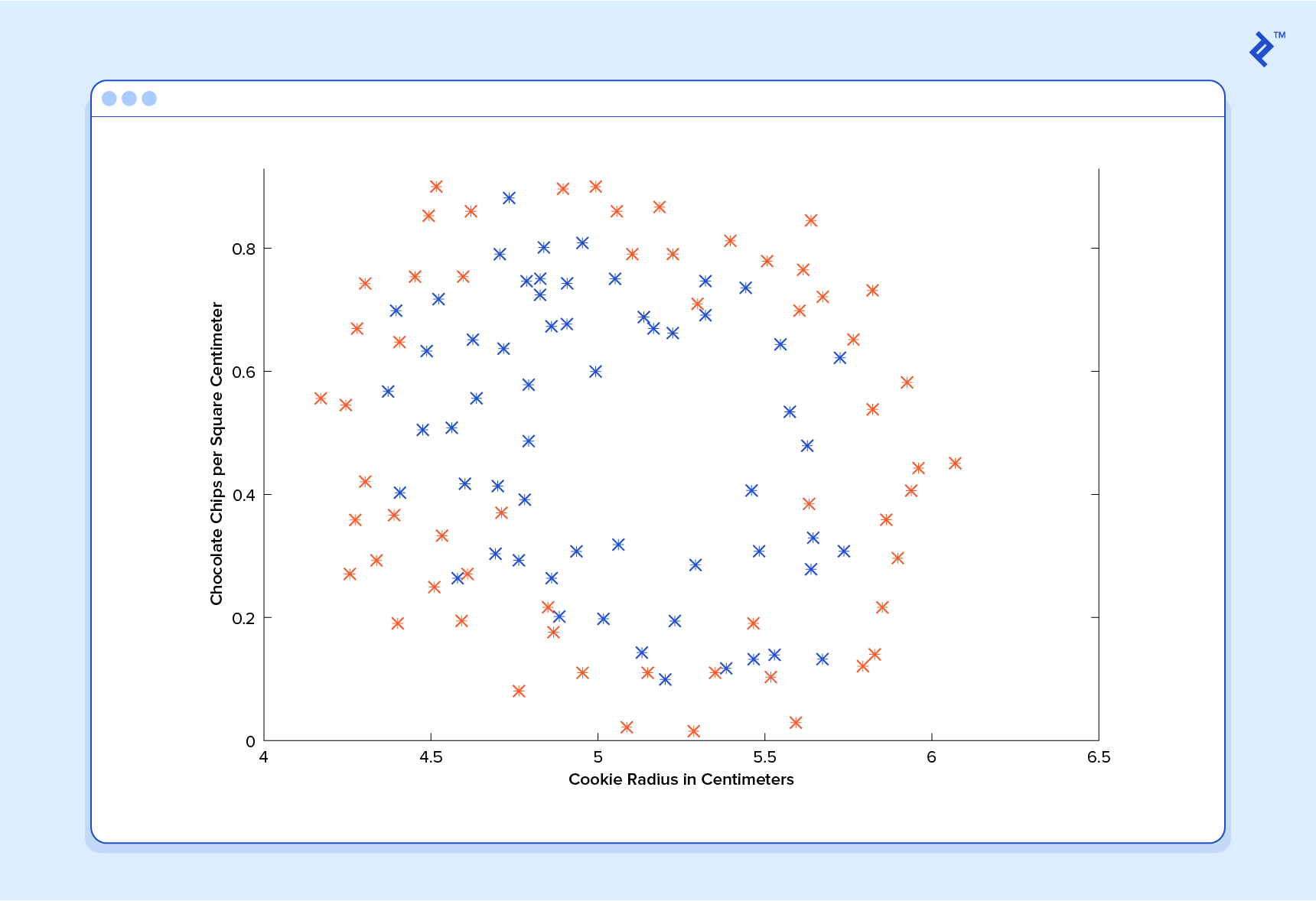
Linear Discriminant Analysis or LDA is an algorithm that provides an indirect approach to solve a classification machine learning problem. To predict the probability, Pn(X) that a given feature, X belongs to a given class Yn or not, it assumes a density function of all the features that belong to that class. It then uses this density function, fn(X) to predict the probability Pn(X) using

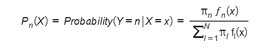
where π_n is the overall or prior probability that a randomly picked observation belongs to nth class.

Let the dataset have only feature variable, then the LDA assumes a Gaussian distribution function for fn(X) having a class-specific mean vector (𝜇n) and a covariance matrix that is applicable for all N classes. After that to assign a class to an observation from the testing data set, it evaluates the discriminant function

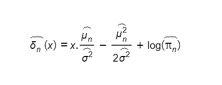
The  LDA classifier then predicts the class of the test variable for which the value of the discriminant function is the largest. We call this algorithm as “linear” discriminant analysis because, in the discriminant function, the component functions are all linear functions of x. 

Note: In the case of more than one variable, LDA assumes a  multivariate gaussian function and the discriminant function is scaled accordingly.

Advantages of Linear Discriminant Analysis

1. It works well for machine learning problems where the classes to be assigned are well-separated.

2. The LDA provides stable results if the number of feature variables in the given dataset is small and fits the normal distribution well.

3. It is easy to understand and simple to use.

Disadvantages of Linear Discriminant Analysis

1. It requires the feature variables to follow the Gaussian distribution and thus has limited applications. 

2. It does not perform very well on datasets having a small number of target variables.

Applications of Linear Discriminant Analysis

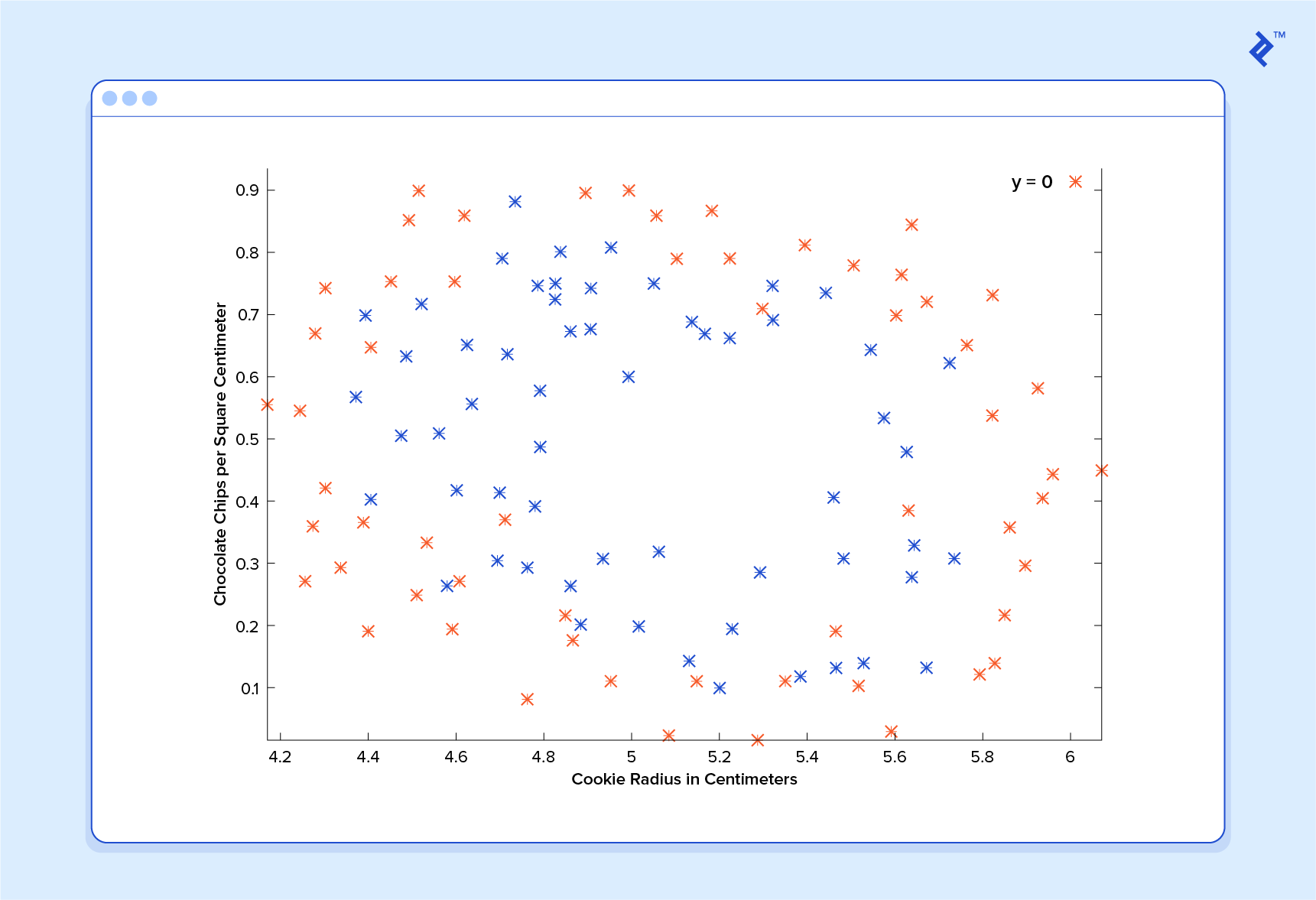
Classifying the Iris Flowers: The famous Iris Dataset contains four features (sepal length, petal length, sepal width, petal width) of three types of Iris flowers. You can use LDA to classify these flowers based on the given four features.

Quadratic Discriminant Analysis

This algorithm is similar to the LDA algorithm that we discussed above. Similar to LDA, the QDA algorithm assumes that feature variables belonging to a particular class obey the gaussian distribution function and utilizes Bayes’ theorem for predicting the covariance matrix.

However, in contrast to LDA, QDA presumes that each class in the target variables has its covariance matrix. And, if one implements this assumption to evaluate the word linear is replaced by quadratic. Learn how to implement this algorithm.

Advantages of Quadratic Discriminant Analysis

1. It performs well for machine learning problems where the size of the training set is large.

2. QDA advises for machine learning problems where the feature variables in the given dataset clearly don’t seem to have a common covariance matrix for N classes. 

3. It helps in deducing the quadratic decision boundary.

4. It servers as a good compromise between the KNN, LDA, and Logistic regression machine learning algorithms.

5. It gives better results when there is non-linearity in the feature variables.

Disadvantages of Quadratic Discriminant Analysis

1. The results are greatly affected if the feature variables do not obey the gaussian distribution function.

2. It performs very well on datasets having feature variables that are uncorrelated.

Applications of Quadratic Discriminant Analysis

Classification of Wine: Yes, one can use the QDA algorithm to learn how to classify wine with Python’s sklearn library.  Check out our free recipe: How to classify wine using sklearn LDA and QDA model? know more.

Perform QDA on Iris Dataset: You can use the Iris Dataset to understand the LDA algorithm and the QDA algorithm. To explore how to do that in detail, check How does Quadratic Discriminant Analysis work?

Principal Component Analysis 

Principal components are the selected feature variables in a large dataset that allow the presentation of almost all the essential information through a smaller number of feature variables. 

And principal component analysis (PCA) is the method by which these principal components are evaluated and used to understand the data better. It is an unsupervised algorithm and thus doesn’t require the input data to have target values. Here is a complete PCA (Principal Component Analysis) Machine Learning Tutorial that you can go through if you want to learn how to implement PCA to solve machine learning problems.

Advantages of Principal Component Analysis

1.  It can be used for visualizing the dataset and can thus be implemented while performing Exploratory Data Analysis. 
2. It is an excellent unsupervised learning method when working with large datasets as it removes correlated feature variables.
3. It assists in saving on computation power.
4. It is one of the commonly used dimensionality reduction algorithms.
5. It reduces the chances of overfitting a dataset.
6. It is also used for factor analysis in statistical learning.

Disadvantages of Principal Component Analysis

1. PCA requires users to normalize their feature variables before implementing them to solve data science problems.

2. As only a subset of feature variables is selected to understand the dataset, the information obtained will likely be incomplete.

Applications of Principal Component Analysis

Below, we have listed two easy applications of PCA for you to practice.

Perform PCA on Digits Dataset: Python’s sklearn library has an inbuilt dataset, ‘digits’, that you can use to understand the implementation of the PCA. Check out our free recipe: How to reduce dimensionality using PCA in Python? to know more.

Apply PCA on Breast Cancer Dataset: Python’s sklearn library has another breast cancer dataset. Check out our free recipe: How to extract features using PCA in Python? To learn how to implement PCA on the breast cancer dataset.

General Additive Models (GAMs) 

GAMs is a more polished and flexible version of the multiple linear regression machine learning model. That is because they support using non-linear functions of each feature variable and still reflect additivity. 

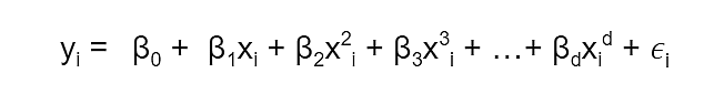
For regression problems, GAMs include the use of formulae like the one given below for predicting target variable, y given the feature variable (xi) :

yi =   êžµ0 +  f1|(xi1) + f2(xi2) + f3(xi3) + …+ fp(xip) + 𝜖i

Where 𝜖i represents the error terms. GAMs are additive as separate functions are evaluated for each feature variable and are then added together. For classification problems, GAMs extend logistic regression to evaluate the probability, 

 p(x) of whether a given feature variable (xi) is an instance of a class (yi) or not.The formula is given by,

log(p(x) / (1-p(x)) = êžµ0 +  f1(x1) + f2(x2) + f3(x3) + …+ fp(xip) + 𝜖i

Advantages of General Additive Models

1. GAMs can be used for both classification and regression problems.

2. They allow modeling of non-linear relationships easily as they require users to manually carry out different transformations on each variable individually manually.

3. Non-linear predictions made using GAMs are relatively accurate.

4. Individual transformations on each feature variable lead to insightful conclusions about each variable in the dataset.

5. They are a practical compromise between linear and fully nonparametric models.

Disadvantages of General Additive Models

1. The model is restricted to be additive and does not support complex interactions among feature variables.

Applications of General Additive Models

You can use the pyGAM library in Python to explore GAMs.

Polynomial Regression

This algorithm is an extension of the linear regression machine learning model. Instead of assuming a linear relation between feature variables (x_i) and the target variable (y_i), it uses a polynomial expression to describe the relationship. The polynomial term used is given by

where 𝜖i represents the error term and d is the polynomial degree. If one uses a large value for d, this algorithm supports estimating non-linear relationships between the feature and target variables.

Advantages of Polynomial Regression

1. It offers a simple method to fit non-linear data. 

2. It is easy to implement and is not computationally expensive

3. It can fit a varied range of curvatures.

4. It makes the pattern in the dataset more interpretable.

Disadvantages of Polynomial Regression

1. Using higher values for the degree of the polynomial supports overly flexible predictions and overfitting.

2. It has a high sensitivity for outliers.

3. It is difficult to predict what degree of the polynomial should be chosen for fitting a given dataset.

Access Data Science and Machine Learning Project Code Examples

Applications of Polynomial Regression

Use Polynomial Regression for Boston Dataset: Python’s sklearn library has the Boston Housing dataset with 13 feature variables and one target variable. One can use Polynomial regression to use the 13 variables to predict the median value of the price of the houses in Boston. If you are curious about how to realize this in Python, check How and when to use polynomial regression? 

FAQs

What are the three types of Machine Learning?

The three types of machine learning are:

1. Unsupervised Machine Learning Algorithms
2. Supervised Machine Learning Algorithms
3. Reinforcement Learning

Which language is the best for machine learning?

Python is considered one of the best programming languages for machine learning as it contains many libraries for efficiently implementing various algorithms in machine learning.

What is the simplest machine learning algorithm?

The simplest machine learning algorithm is linear regression. It is a simple algorithm that spans different domains. For example, it is used in Physics to evaluate the spring constant of a spring using Hooke’s law.

What are algorithms in machine learning?

Algorithms in machine learning are the mathematical equations that help understand the relationship between a given set of feature variables and dependent variables. Using these equations, one can predict the value of the dependent variable.

Which algorithm is best for machine learning?

The best algorithms in machine learning are the algorithms that help you understand your data the best and draw efficient predictions from it.

What are the common machine learning algorithms?

The common machine learning algorithms are: 

• Random Forest
• Decision trees
• Neural networks
• Logistic regression
• Linear regression

Machine learning is a type of AI that teaches machines how to learn, interpret and predict results based on a set of data. As the world — and internet — have grown exponentially in the past few years, machine learning processes have become common for organizations of all kinds. For example, companies in the healthcare sector use ML to detect and treat diseases better, while in the farming sector machine learning helps predict harvest yields.

ML involves computers finding insightful information without being told where to look, differing so from traditional computing, in which algorithms are sets of explicitly programmed instructions. ML does this by leveraging algorithms that are trained on data, on which they learn in an iterative process in order to generate outputs, and automate decision-making processes.

The three basic ingredient of machine learning

There are three basic functional ingredients of ML.

1. Data: The dataset you want to use must be well-structured, accurate. The data you use can be labeled or unlabeled. Unlabeled data are sample items — e.g. photos, videos, news articles — that don’t need additional explanation, while labeled ones are augmented: unlabeled information is bundled and an explanation, with a tag, is added to them.
2. Algorithm: there are different types of algorithms that can be used (e.g. linear regression, logistic regression). Choosing the right algorithm is both a combination of business need, specification, experimentation and time available.
3. Model: ​​A “model” is the output of a machine learning algorithm run on data. It represents the rules, numbers, and any other algorithm-specific data structures required to make predictions.

How is machine learning used

Successful machine learning algorithms can be used for a variety of purposes. The Director of the Massachusetts Institute of Technology (MIT), Thomas W. Malone wrote in a recent research:

“ The function of a machine learning system can be descriptive, meaning that the system uses the data to explain what happened; predictive, meaning the system uses the data to predict what will happen; or prescriptive, meaning the system will use the data to make suggestions about what action to take.”

What are training data

Training data is the initial data used to train machine learning models. Training datasets are fed to machine learning algorithms so that they can learn to make predictions, or perform a desired task. This type of data is key, because it helps machines achieve results and work in the right way, as shown in the graph below.

‍

‍

The innovative power of machine learning models is in the fact that they learn and improve over time, as they are exposed to relevant training data. Some data is held out from the training data to be used as “evaluation data ‘’, which validates and tests how accurate the machine learning model is. This type of data is contained in the validation and test datasets which will be later discussed.

The importance of training data

Training data is a key part of the machine learning process. There are several aspects in play when you build a training dataset. The prime consideration is the size of datasets which depends on the use made of ML: More complicated the use, the bigger the size of the dataset. In the case of unsupervised learning, the more patterns you want your model to identify, the more examples it will need. You want a scalable learning algorithm, which can deal with any amount of data.

Second thing to consider is the quality of the data. Concerning this aspect, it is important to feed the system with carefully curated data. The higher the quality of your training data is, the better will your machine learning model be, especially in the early stages.

Having quality in data you used, means collecting real-world data, which closely mimics how an application will receive external inputs, and diverse data, for reducing the possibility of biases that we will later discuss.

To understand how much training data is important, think of vehicle manufacturers that are pivoting themselves towards the challenge of autonomous drive. The quality of the data is essential to ensuring autonomous vehicles operate safely and as expected. It isn’t enough for vehicles to perform well in simulated-good weather conditions, or on one type of road. They must perform flawlessly in all weather conditions in every imaginable road scenario.

Keep also in mind that the quality of the data comes from including the final user in your product/service. The most successful AI projects are those that integrate data collection during the product life-cycle. It must be built into the core of the product itself, in order that every time a user engages with it, you collect data from that interaction. The main purpose is to use the constant data flow to improve your offer for the user. Think of Spotify that uses an AI system called “collaborative filtering”, to create personalized “Discover Weekly” playlists which help fans to sort out new music that’s appealing to them. The more the user listens to and searches for music that he/she enjoys, the more the app will know what to recommend.

How machine learning can learn from data

Machine learning offers a number of different ways to learn from data:

• Supervised learning : it can be regarded as a “hands-on” approach, since it uses labeled data. Humans must tag, label, or annotate the data to their criteria, in order to train the model to predict the “correct” outputs which are predetermined.
• Unsupervised learning : it can be construed as a “broad pattern-seeking” approach, since it uses unlabeled data and, instead of predicting the correct output, models are tasked with finding patterns, similarities and deviations, that can be then applied to other data that exhibit similar behaviour.
• Reinforcement learning: it uses unlabeled data and it involves a feedback mechanism. When it performs a task correctly, it receives positive feedback, which strengthens the model in connecting the target inputs and output. Likewise, it can receive negative feedback for incorrect solutions.

Validation and testing

Validation and testing begins with splitting your training dataset. The “Valid-Test split” is a technique to evaluate the performance of your ML model. You need to split the data because you don’t want your model to over-learn from training data, to not perform well. But, most of all, you want to evaluate how well your model is generalizing.

Hence, you held back from training dataset, validation and testing subsets for assessing your model in a meaningful way. Notice that a typical split ratio of data, between training, validation and testing sets is around 50:25:25. A brief explanation of the role of each of these dataset is below.

• Validation dataset: it is useful when it comes to model selection. The data included in this set will be used to find the optimal values for the parameters of the model under consideration. When you work with ML models, you typically need to test multiple models with different parameters values for finding the optimal values that will give the best possible performance. Therefore, in order to pick the best model you must evaluate each of them.
• Testing dataset: when you have tuned the model by performing parameters optimisation, you should end up with the final model. The testing set is used to provide an unbiased evaluation of the performance of this model and ensure that it can generalise well to new, unseen data.

‍

‍

Bias in machine learning

Bias in Machine Learning is defined as the phenomena of observing results that are systematically prejudiced due to faulty assumptions. It can be interpreted as the accuracy of our predictions. A high bias will result in an inaccurate prediction, so you need to know what bias is, to prevent it. An inaccurate prediction can derive from

There are techniques to handle bias, and they are related to the quality of training data. For sure, they must be as diverse as possible, including as many relevant groups of data as possible. The more inclusive is the dataset, the less likely it is to turn a blind eye to a given data group. You must identify representative data.

In general, bias reduces the potential of AI for business and society by encouraging mistrust and producing distorted results. Any value delivered by machine learning systems in terms of efficiency or productivity will be wiped out if the algorithms discriminate against individuals.

What are the different types of bias in Machine Learning

• Sample bias: if the sample data used to train models do not replicate a real-world scenario, models are exposed to a part of the problem space. An example is facial recognition softwares primarily trained on images of white men.
• Prejudicial bias: it occurs due to cultural stereotypes. Social status and gender may slide into a model. The consequence is that results will be skewed against people of a particular group. When a software used to hire talents, is fed mostly male resumes, it will learn that men are preferable to other profiles
• Algorithmic bias: it may occur when the algorithm used is inappropriate for the current application. It is an error that derives from an error of approach. This bias can emerge due to the wrong “architectural” design of the algorithm or to unintentional decisions relating to the way data is collected. It is quite difficult to address.
• Exclusion bias: it happens when important data are excluded from the training dataset. For example, imagine you have a dataset of customer sales in America and Europe. 98% of the customers are from America, so you choose to delete the location data thinking it is irrelevant. This means your model will not pick up on the fact that your European customers spend two times more.

How businesses are using machine learning

Every company is pivoting to use machine learning in their products and services in some way. It is almost like ML is becoming an expected feature. We are using it to make human tasks easier, faster, and better than before.

As said in the introduction, an example of Machine Learning applied to content consumption is Netflix with its personalisation of movie recommendations, in order to “learn to entertain the world”. Users who watch A are likely to watch B. Netflix uses the watching history of other users with similar tastes to recommend what you may be most interested in watching next.

Product recommendation is one of the most successful applications of machine learning in business. They will pull in front of you those products you are most likely to buy, according to the product you have previously bought and browsed. For example, Amazon uses the browsing history of a user to always keep those products in the customer’s sight.

Machine learning is also used by advertisers, for the so called “machine learning based advertising”. Using ML in this field is fundamental especially because of the changes introduced by Apple updates for iOS. Privacy is a key feature of them, and this made for marketers the optimization of the ROI of their campaigns even harder, since precise targeting has become difficult. As advertising gets more complex, you need to rely on the analytical and on real-time optimisation capacities that an algorithm can provide.

Here at Mapendo, Jenga, our proprietary AI technology, collects tens of thousands of data related to a given topic, finds patterns, and it manages to predict the possible outcome of a marketing campaign and finds the audience that is most likely to convert for a type of ad.

Our algorithm has been trained to optimize the traffic according to the client’s KPIs, maximize user retention and generate post install actions. Advertisers need to leverage technology to find meaningful insights, predict outcomes and maximise the efficiency of their investment, by choosing the right channels and budget.

Conclusion

A basic understanding of machine learning is important. This is for two reasons. The first one is that ML can really improve our life, finding applications in our daily routines. Instead, the second one is that with digitalisation disrupting every industry, sharing and delivering data has become a high priority.

As we have explained it is fundamental to build a trained model. For guaranteeing a quality “coaching”, you must provide machine learning with accurate data, and in the right amounts. The way you teach the algorithm and how it learns, depends on how much accuracy it is put into constructing your dataset, inputting labeled or unlabeled data, and paying close attention to not feed the algorithm with biased ones. Data biases will lead to unreliable results, and if you use those, you will give the wrong answer to your problem. Biased datasets can jeopardize business processes and decisions.

The last fundamental step is the one that leads to the final results of the machine learning process. Validation and, in greater detail, testing will determine the overall model performance, making sure that the model can really work when you use it to give an answer to a real-world problem.

What is Machine Learning?

A subset of artificial intelligence (AI) and computer science, machine learning (ML) deals with the study and use of data and algorithms that mimic how humans learn. This helps machines gradually improve their accuracy. ML allows software applications to improve their prediction accuracy without being specifically programmed to do so. It estimates new output values by using historical data as input.

Importance of Machine Learning

In today’s technological era, machine learning has become an integral part of diverse industries and sectors. It is extremely important because it provides organisations with insights into trends in customer behaviour and business operating patterns, as well as assisting in the creation of new products. Machine learning is fundamental to the operations of many of today’s biggest organisations, like Facebook, Google, and Uber. For many businesses across the world, it has become a crucial competitive differentiator.

Types of Machine Learning

Machine learning algorithms are broadly divided into four types – supervised learning, unsupervised learning, semi-supervised learning, and reinforcement learning.

Supervised Learning    

In the case of supervised learning, machines are trained by examples. The machine is taught by example in supervised learning. The operator gives the machine learning algorithm a predefined dataset with specified inputs and outputs, and the algorithm needs to figure out how to get those inputs and outputs. While the operator is aware of the proper responses, the algorithm recognises patterns in data, learns from observations, and produces predictions. The algorithm predicts and is corrected by the operator; this process is repeated till the algorithm reaches a high level of precision.

Unsupervised Learning

The machine learning programme examines the data to detect trends. There is no response key or human interference to provide guidance. Instead, the machine analyses available data to discover correlations and linkages. The machine learning algorithm is left to evaluate massive data sets and address that data in an unsupervised learning process. The programme attempts to organise the data in a way that describes its structure. This could imply organizing the data into clusters or structuring it in a more organised manner. As it evaluates additional data, its capability to make decisions based on that data increases and gets more refined.

Semi-Supervised Learning        

It is akin to supervised learning but it employs both labelled and unlabelled data. Labelled data is mainly information that has semantic tags so that the algorithm can interpret it, but unlabelled data does not have that information. Machine learning systems can learn to categorise unlabelled data using this combination.

Reinforcement Learning

Reinforcement learning is concerned with regimented learning procedures in which a machine learning algorithm is given a set of actions, variables, and end values to follow. Following the definition of the rules, the algorithm attempts to explore several options and prospects, monitoring and assessing each output to determine which is ideal. Reinforcement learning instructs the machine through trial and error. It learns from previous experiences and begins to change its approach to the situation to reach the best possible outcome.

Applications of Machine Learning

Some of the applications of machine learning include:

• Recommendation engines
• Business process automation
• Spam filtering
• Malware threat detection
• Predictive maintenance
• Virtual personal assistant
• Medical diagnosis
• Stock market trading
• Speech and image recognition
• Self-driving cars

And the list goes on and on. Today, machine learning is at the heart of many real-world applications.

There are many institutions such as the FORE School of Management that are offering machine learning courses in Delhi NCR. The future of machine learning is promising and if you want to make a career in this domain, enrol in a course today to obtain a valid credential.

Machine learning offers new opportunities, but with power comes responsibility – ethical considerations cannot be ignored.

Machine learning (ML) is a sub-set of artificial intelligence (AI). It is generally understood as the ability of the system to make predictions or draw conclusions based on the analysis of a large historical data set.

The exponential increase in the availability of data, and unprecedented computing power for processing this data, have contributed to moving AI from fiction to fact.

AI means a lot of different things to different people and a wide range of terms are usually involved when talking about it. Broadly speaking, there are two levels of AI – specific/weak and general. Most business applications involving machine learning refer to weak AI. In order to make sense of the AI landscape, it can be helpful to learn what the different terms refer to.

ML is being increasingly used in accounting software and business process applications. And as a finance professional it is important to develop an appreciation of all this.

Ethical considerations

Professional accountants need to consider, and appropriately manage, potential ethical compromises that may result from decision making by an algorithm. They must remain engaged in AI and its component parts, including machine learning.

The ethical challenges posed by ML are explored in this section by focusing on five areas:

• Dealing with bias
• Strategic view of data
• Assigning accountability 
• Looking beyond the hype
• Acting in the public interest

Skills in a machine learning environment

The ability of AI to take over jobs is a narrative often recited in the media. And there is certainly some truth about the ability of these technologies to do a variety of tasks more efficiently.

But even sophisticated technology such as AI struggles to replicate the full contextual understanding and integrated thinking of which humans are capable.

Now is a good time to start building greater knowledge and awareness in this area. The technology has moved beyond unrealistic fantasy to real business applications. Some will embrace it. Others will fear it. But only the reckless will avoid finding out more about it.

It’s no longer the preserve of artificial-intelligence researchers and born-digital companies like Amazon, Google, and Netflix.

Machine learning is based on algorithms that can learn from data without relying on rules-based programming. It came into its own as a scientific discipline in the late 1990s as steady advances in digitization and cheap computing power enabled data scientists to stop building finished models and instead train computers to do so. The unmanageable volume and complexity of the big data that the world is now swimming in have increased the potential of machine learning—and the need for it.

In 2007 Fei-Fei Li, the head of Stanford’s Artificial Intelligence Lab, gave up trying to program computers to recognize objects and began labeling the millions of raw images that a child might encounter by age three and feeding them to computers. By being shown thousands and thousands of labeled data sets with instances of, say, a cat, the machine could shape its own rules for deciding whether a particular set of digital pixels was, in fact, a cat.¹ Last November, Li’s team unveiled a program that identifies the visual elements of any picture with a high degree of accuracy. IBM’s Watson machine relied on a similar self-generated scoring system among hundreds of potential answers to crush the world’s best Jeopardy! players in 2011.

Dazzling as such feats are, machine learning is nothing like learning in the human sense (yet). But what it already does extraordinarily well—and will get better at—is relentlessly chewing through any amount of data and every combination of variables. Because machine learning’s emergence as a mainstream management tool is relatively recent, it often raises questions. In this article, we’ve posed some that we often hear and answered them in a way we hope will be useful for any executive. Now is the time to grapple with these issues, because the competitive significance of business models turbocharged by machine learning is poised to surge. Indeed, management author Ram Charan suggests that “any organization that is not a math house now or is unable to become one soon is already a legacy company.²

1. How are traditional industries using machine learning to gather fresh business insights?

Well, let’s start with sports. This past spring, contenders for the US National Basketball Association championship relied on the analytics of Second Spectrum, a California machine-learning start-up. By digitizing the past few seasons’ games, it has created predictive models that allow a coach to distinguish between, as CEO Rajiv Maheswaran puts it, “a bad shooter who takes good shots and a good shooter who takes bad shots”—and to adjust his decisions accordingly.

You can’t get more venerable or traditional than General Electric, the only member of the original Dow Jones Industrial Average still around after 119 years. GE already makes hundreds of millions of dollars by crunching the data it collects from deep-sea oil wells or jet engines to optimize performance, anticipate breakdowns, and streamline maintenance. But Colin Parris, who joined GE Software from IBM late last year as vice president of software research, believes that continued advances in data-processing power, sensors, and predictive algorithms will soon give his company the same sharpness of insight into the individual vagaries of a jet engine that Google has into the online behavior of a 24-year-old netizen from West Hollywood.

2. What about outside North America?

In Europe, more than a dozen banks have replaced older statistical-modeling approaches with machine-learning techniques and, in some cases, experienced 10 percent increases in sales of new products, 20 percent savings in capital expenditures, 20 percent increases in cash collections, and 20 percent declines in churn. The banks have achieved these gains by devising new recommendation engines for clients in retailing and in small and medium-sized companies. They have also built microtargeted models that more accurately forecast who will cancel service or default on their loans, and how best to intervene.

Closer to home, as a recent article in McKinsey Quarterly notes,³ our colleagues have been applying hard analytics to the soft stuff of talent management. Last fall, they tested the ability of three algorithms developed by external vendors and one built internally to forecast, solely by examining scanned résumés, which of more than 10,000 potential recruits the firm would have accepted. The predictions strongly correlated with the real-world results. Interestingly, the machines accepted a slightly higher percentage of female candidates, which holds promise for using analytics to unlock a more diverse range of profiles and counter hidden human bias.

As ever more of the analog world gets digitized, our ability to learn from data by developing and testing algorithms will only become more important for what are now seen as traditional businesses. Google chief economist Hal Varian calls this “computer kaizen.” For “just as mass production changed the way products were assembled and continuous improvement changed how manufacturing was done,” he says, “so continuous [and often automatic] experimentation will improve the way we optimize business processes in our organizations.”⁴

3. What were the early foundations of machine learning?

Machine learning is based on a number of earlier building blocks, starting with classical statistics. Statistical inference does form an important foundation for the current implementations of artificial intelligence. But it’s important to recognize that classical statistical techniques were developed between the 18th and early 20th centuries for much smaller data sets than the ones we now have at our disposal. Machine learning is unconstrained by the preset assumptions of statistics. As a result, it can yield insights that human analysts do not see on their own and make predictions with ever-higher degrees of accuracy.

More recently, in the 1930s and 1940s, the pioneers of computing (such as Alan Turing, who had a deep and abiding interest in artificial intelligence) began formulating and tinkering with the basic techniques such as neural networks that make today’s machine learning possible. But those techniques stayed in the laboratory longer than many technologies did and, for the most part, had to await the development and infrastructure of powerful computers, in the late 1970s and early 1980s. That’s probably the starting point for the machine-learning adoption curve. New technologies introduced into modern economies—the steam engine, electricity, the electric motor, and computers, for example—seem to take about 80 years to transition from the laboratory to what you might call cultural invisibility. The computer hasn’t faded from sight just yet, but it’s likely to by 2040. And it probably won’t take much longer for machine learning to recede into the background.

4. What does it take to get started?

C-level executives will best exploit machine learning if they see it as a tool to craft and implement a strategic vision. But that means putting strategy first. Without strategy as a starting point, machine learning risks becoming a tool buried inside a company’s routine operations: it will provide a useful service, but its long-term value will probably be limited to an endless repetition of “cookie cutter” applications such as models for acquiring, stimulating, and retaining customers.

We find the parallels with M&A instructive. That, after all, is a means to a well-defined end. No sensible business rushes into a flurry of acquisitions or mergers and then just sits back to see what happens. Companies embarking on machine learning should make the same three commitments companies make before embracing M&A. Those commitments are, first, to investigate all feasible alternatives; second, to pursue the strategy wholeheartedly at the C-suite level; and, third, to use (or if necessary acquire) existing expertise and knowledge in the C-suite to guide the application of that strategy.

The people charged with creating the strategic vision may well be (or have been) data scientists. But as they define the problem and the desired outcome of the strategy, they will need guidance from C-level colleagues overseeing other crucial strategic initiatives. More broadly, companies must have two types of people to unleash the potential of machine learning. “Quants” are schooled in its language and methods. “Translators” can bridge the disciplines of data, machine learning, and decision making by reframing the quants’ complex results as actionable insights that generalist managers can execute.

Access to troves of useful and reliable data is required for effective machine learning, such as Watson’s ability, in tests, to predict oncological outcomes better than physicians or Facebook’s recent success teaching computers to identify specific human faces nearly as accurately as humans do. A true data strategy starts with identifying gaps in the data, determining the time and money required to fill those gaps, and breaking down silos. Too often, departments hoard information and politicize access to it—one reason some companies have created the new role of chief data officer to pull together what’s required. Other elements include putting responsibility for generating data in the hands of frontline managers.

Start small—look for low-hanging fruit and trumpet any early success. This will help recruit grassroots support and reinforce the changes in individual behavior and the employee buy-in that ultimately determine whether an organization can apply machine learning effectively. Finally, evaluate the results in the light of clearly identified criteria for success.

5. What’s the role of top management?

Behavioral change will be critical, and one of top management’s key roles will be to influence and encourage it. Traditional managers, for example, will have to get comfortable with their own variations on A/B testing, the technique digital companies use to see what will and will not appeal to online consumers. Frontline managers, armed with insights from increasingly powerful computers, must learn to make more decisions on their own, with top management setting the overall direction and zeroing in only when exceptions surface. Democratizing the use of analytics—providing the front line with the necessary skills and setting appropriate incentives to encourage data sharing—will require time.

C-level officers should think about applied machine learning in three stages: machine learning 1.0, 2.0, and 3.0—or, as we prefer to say, description, prediction, and prescription. They probably don’t need to worry much about the description stage, which most companies have already been through. That was all about collecting data in databases (which had to be invented for the purpose), a development that gave managers new insights into the past. OLAP—online analytical processing—is now pretty routine and well established in most large organizations.

There’s a much more urgent need to embrace the prediction stage, which is happening right now. Today’s cutting-edge technology already allows businesses not only to look at their historical data but also to predict behavior or outcomes in the future—for example, by helping credit-risk officers at banks to assess which customers are most likely to default or by enabling telcos to anticipate which customers are especially prone to “churn” in the near term (exhibit).

Exhibit

We strive to provide individuals with disabilities equal access to our website. If you would like information about this content we will be happy to work with you. Please email us at: McKinsey_Website_Accessibility@mckinsey.com

A frequent concern for the C-suite when it embarks on the prediction stage is the quality of the data. That concern often paralyzes executives. In our experience, though, the last decade’s IT investments have equipped most companies with sufficient information to obtain new insights even from incomplete, messy data sets, provided of course that those companies choose the right algorithm. Adding exotic new data sources may be of only marginal benefit compared with what can be mined from existing data warehouses. Confronting that challenge is the task of the “chief data scientist.”

Prescription—the third and most advanced stage of machine learning—is the opportunity of the future and must therefore command strong C-suite attention. It is, after all, not enough just to predict what customers are going to do; only by understanding why they are going to do it can companies encourage or deter that behavior in the future. Technically, today’s machine-learning algorithms, aided by human translators, can already do this. For example, an international bank concerned about the scale of defaults in its retail business recently identified a group of customers who had suddenly switched from using credit cards during the day to using them in the middle of the night. That pattern was accompanied by a steep decrease in their savings rate. After consulting branch managers, the bank further discovered that the people behaving in this way were also coping with some recent stressful event. As a result, all customers tagged by the algorithm as members of that microsegment were automatically given a new limit on their credit cards and offered financial advice.

The prescription stage of machine learning, ushering in a new era of man–machine collaboration, will require the biggest change in the way we work. While the machine identifies patterns, the human translator’s responsibility will be to interpret them for different microsegments and to recommend a course of action. Here the C-suite must be directly involved in the crafting and formulation of the objectives that such algorithms attempt to optimize.

6. This sounds awfully like automation replacing humans in the long run. Are we any nearer to knowing whether machines will replace managers?

It’s true that change is coming (and data are generated) so quickly that human-in-the-loop involvement in all decision making is rapidly becoming impractical. Looking three to five years out, we expect to see far higher levels of artificial intelligence, as well as the development of distributed autonomous corporations. These self-motivating, self-contained agents, formed as corporations, will be able to carry out set objectives autonomously, without any direct human supervision. Some DACs will certainly become self-programming.

One current of opinion sees distributed autonomous corporations as threatening and inimical to our culture. But by the time they fully evolve, machine learning will have become culturally invisible in the same way technological inventions of the 20th century disappeared into the background. The role of humans will be to direct and guide the algorithms as they attempt to achieve the objectives that they are given. That is one lesson of the automatic-trading algorithms which wreaked such damage during the financial crisis of 2008.

No matter what fresh insights computers unearth, only human managers can decide the essential questions, such as which critical business problems a company is really trying to solve. Just as human colleagues need regular reviews and assessments, so these “brilliant machines” and their works will also need to be regularly evaluated, refined—and, who knows, perhaps even fired or told to pursue entirely different paths—by executives with experience, judgment, and domain expertise.

The winners will be neither machines alone, nor humans alone, but the two working together effectively.

7. So in the long term there’s no need to worry?

It’s hard to be sure, but distributed autonomous corporations and machine learning should be high on the C-suite agenda. We anticipate a time when the philosophical discussion of what intelligence, artificial or otherwise, might be will end because there will be no such thing as intelligence—just processes. If distributed autonomous corporations act intelligently, perform intelligently, and respond intelligently, we will cease to debate whether high-level intelligence other than the human variety exists. In the meantime, we must all think about what we want these entities to do, the way we want them to behave, and how we are going to work with them.

The goal of machine learning is to train machines to get better at tasks without explicit programming. To achieve this goal, several steps have to take place. First, data needs to be collected and prepared. Then, a training model, or algorithm, needs to be selected. After which, the model needs to be evaluated so that hyperparameter tuning can happen and predictions can be made. It’s also important to note that there are different types of machine learning which include supervised learning, unsupervised learning, semi-supervised learning, and reinforcement learning.

Machine Learning vs. Traditional Programming

Machine learning is when both data and output are run on a computer to create a program that can then be used in traditional programming. And traditional programming is when data and a program are run on a computer to produce an output. Whereas traditional programming is a more manual process, machine learning is more automated. As a result, machine learning helps to increase the value of embedded analytics, speeds up user insights, and reduces decision bias.

Machine Learning and Artificial Intelligence

While machine learning is a subset of artificial intelligence, it has its differences. For instance, machine learning trains machines to improve at tasks without explicit programming, while artificial intelligence works to enable machines to think and make decisions just as a human would.

Machine Learning and Deep Learning

Deep learning is a subset of machine learning, and it uses multi-layered or neural networks for machine learning. Deep learning is well-known for its applications in image and speech recognition as it works to see complex patterns in large amounts of data.

What are the key elements of machine learning?

There are three main elements to every machine learning algorithm, and they include:

• Representation: what the model looks like; how knowledge is represented
• Evaluation: how good models are differentiated; how programs are evaluated 
• Optimization: the process for finding good models; how programs are generated

What are some machine learning applications?

Machine learning helps software applications become even more accurate at predicting outcomes without being explicitly programmed. More and more industries are employing machine learning in the following ways:

• Web search and ranking pages based on search preferences.
• Evaluating risk in finance on credit offers and knowing where is best to invest. 
• Predicting customer churn in e-commerce.
• Space exploration and sending probes to space.
• The advance in robotics and autonomous, self-driving cars.
• Extracting data on relationships and preferences from social media.
• Speeding up the debugging process in computer science.

How does machine learning work?

When it comes to the different types of machine learning, supervised learning and unsupervised learning play key roles. While supervised learning uses a set of input variables to predict the value of an output variable, unsupervised learning discovers patterns within data to better understand and identify like groups within a given dataset.

Supervised Learning

Supervised learning is the most common type of machine learning and is used by most machine learning algorithms. This type of learning, also known as inductive learning, includes regression and classification. Regression is when the variable to predict is numerical, whereas classification is when the variable to predict is categorical. For example, regression would use age to predict income, while classification would use age to predicate a category like making a specific purchase.

Within supervised learning, various algorithms are used, including:

• Linear regression
• Logistic regression
• Decision trees
• Random forest
• Gradient boosting
• Artificial neural networks

Unsupervised Learning

Unsupervised learning is useful when it comes to identifying structure in data. There are many situations when it can be near impossible to identify trends in data, and unsupervised learning is able to provide patterns in data which helps to inform better insights. The common type of algorithm used in unsupervised learning is K-Means or clustering.

What is there to consider when it comes to machine learning?

With machine learning, you want to understand the basics, and you also want to be aware of the algorithms that underpin machine learning. To get started, you want to:

• Collect and prepare data
• Choose a training model or algorithm 
• Evaluate a model
• Hyperparameter tune 
• Make predictions

Domo has created a Machine Learning playbook that anyone can use to properly prepare data, run a model in a ready-made environment, and visualize it back in Domo to simplify and streamline this process. Since building and choosing a model can be time-consuming, there is also automated machine learning (AutoML) to consider. AutoML helps to pre-process data, choose a model, and hyperparameter tune.

Domo’s ETL tools, which are built into the solution, help integrate, clean, and transform data–one of the most challenging parts of the data-to-analyzation process.

How do businesses use machine learning basics?

Machine learning helps businesses reach their desired outcomes faster. Machine learning can help businesses improve efficiencies and operations, do preventative maintenance, adapt to changing market conditions, and leverage consumer data to increase sales and improve retention. Machine learning is even being used across different industries ranging from agriculture to medical research. And when combined with artificial intelligence, machine learning can provide insights that can propel a company forward.

What does the future hold for machine learning?

There are countless opportunities for machine learning to grow and evolve with time. Improvements in unsupervised learning algorithms will most likely be seen contributing to more accurate analysis, which will inform better insights. Since machine learning currently helps companies understand consumers’ preferences, more marketing teams are beginning to adopt artificial intelligence and machine learning to continue to improve their personalization strategies. Additionally, machine learning and deep learning are going to evolve. For instance, with the continual advancements in natural language processing (NLP), search systems can now understand different kinds of searches and provide more accurate answers. All in all, machine learning is only going to get better with time, helping to support growth and increase business outcomes.

Machine learning is a subset of artificial intelligence (AI) in which algorithms learn by example from historical data to predict outcomes and uncover patterns not easily spotted by humans. For example, machine learning can reveal customers who are likely to churn, likely fraudulent insurance claims, and more. While machine learning has been around since the 1950s, recent breakthroughs in low-cost compute resources like cloud storage, easier data collection, and the proliferation of data science have made it very much “the next big thing” in business analytics.

To put it simply, the machine learning algorithm learns by example, and then users apply those self-learning algorithms to uncover insights, determine relationships, and make predictions about future trends. Machine learning has practical implications across industry sectors, including healthcare, insurance, energy, marketing, manufacturing, financial technology (fintech), and more. When implemented effectively, machine learning allows businesses to uncover optimal solutions to practical problems, which leads to real, tangible business value.

Why is Machine Learning Important?

While most statistical analysis relies on rule-based decision-making, machine learning excels at tasks that are hard to define with exact step-by-step rules. Machine learning can be applied to numerous business scenarios in which an outcome depends on hundreds of factors — factors that are difficult or impossible for a human to monitor. As a result, businesses use machine learning for predicting loan defaults, understanding factors that lead to customer churn, identifying likely fraudulent transactions, optimizing insurance claims processes, predicting hospital readmission, and many other cases.

Companies that effectively implement machine learning and other AI technologies gain a massive competitive advantage. According to a recent report by McKinsey & Company, AI technologies will create $50 trillion of value by the year 2025. Companies that fail to do the same will be unable to compete with those who embrace the new frontier – and sooner rather than later.

Machine Learning + DataRobot

Historically, machine learning has been a tedious process that requires a lot of manual coding, limiting the ability of organizations to take full advantage of the technology. Without teams of difficult-to-find data scientists at their disposal, companies are limited in the number of models they are able to develop and test – and often those models take so long to develop, they are outdated by the time they are complete.

To solve this problem, DataRobot invented automated machine learning. Building a high-quality machine learning model often involves a combination of elaborate feature engineering, a Ph.D.-level knowledge of statistics, and extensive software engineering experience. DataRobot strives to make machine learning more accessible to everyone in every organization by incorporating the knowledge and best practices of the world’s best data scientists into a fully automated modeling platform that you can use regardless of data science experience or coding knowledge, delivering insights an order of magnitude faster than was previously possible.

Learn More About AI

• End-to-End AI: The Complete Guide to DataRobot’s Enterprise AI Platform
• DataRobot Documentation: Modeling
• Webinar: Automated Machine Learning in Action
• Ebook: Accelerate the Impact of AI

What is a machine learning Model?

A machine learning model is a program that can find patterns or make decisions from a previously unseen dataset. For example, in natural language processing, machine learning models can parse and correctly recognize the intent behind previously unheard sentences or combinations of words. In image recognition, a machine learning model can be taught to recognize objects – such as cars or dogs. A machine learning model can perform such tasks by having it ‘trained’ with a large dataset. During training, the machine learning algorithm is optimized to find certain patterns or outputs from the dataset, depending on the task. The output of this process – often a computer program with specific rules and data structures – is called a machine learning model.

What is a machine learning Algorithm?

A machine learning algorithm is a mathematical method to find patterns in a set of data. Machine Learning algorithms are often drawn from statistics, calculus, and linear algebra. Some popular examples of machine learning algorithms include linear regression, decision trees, random forest, and XGBoost.

What is Model Training in machine learning?

The process of running a machine learning algorithm on a dataset (called training data) and optimizing the algorithm to find certain patterns or outputs is called model training. The resulting function with rules and data structures is called the trained machine learning model.

What are the different types of Machine Learning?

In general, most machine learning techniques can be classified into supervised learning, unsupervised learning, and reinforcement learning.

What is Supervised Machine Learning?

In supervised machine learning, the algorithm is provided an input dataset, and is rewarded or optimized to meet a set of specific outputs. For example, supervised machine learning is widely deployed in image recognition, utilizing a technique called classification. Supervised machine learning is also used in predicting demographics such as population growth or health metrics, utilizing a technique called regression.

What is Unsupervised Machine Learning?

In unsupervised machine learning, the algorithm is provided an input dataset, but not rewarded or optimized to specific outputs, and instead trained to group objects by common characteristics. For example, recommendation engines on online stores rely on unsupervised machine learning, specifically a technique called clustering.

What is Reinforcement Learning?

In reinforcement learning, the algorithm is made to train itself using many trial and error experiments. Reinforcement learning happens when the algorithm interacts continually with the environment, rather than relying on training data. One of the most popular examples of reinforcement learning is autonomous driving.

What are the different machine learning models?

There are many machine learning models, and almost all of them are based on certain machine learning algorithms. Popular classification and regression algorithms fall under supervised machine learning, and clustering algorithms are generally deployed in unsupervised machine learning scenarios.

Supervised Machine Learning

• Logistic Regression: Logistic Regression is used to determine if an input belongs to a certain group or not
• SVM: SVM, or Support Vector Machines create coordinates for each object in an n-dimensional space and uses a hyperplane to group objects by common features
• Naive Bayes: Naive Bayes is an algorithm that assumes independence among variables and uses probability to classify objects based on features
• Decision Trees: Decision trees are also classifiers that are used to determine what category an input falls into by traversing the leaf’s and nodes of a tree
• Linear Regression: Linear regression is used to identify relationships between the variable of interest and the inputs, and predict its values based on the values of the input variables.
• kNN: The k Nearest Neighbors technique involves grouping the closest objects in a dataset and finding the most frequent or average characteristics among the objects.
• Random Forest: Random forest is a collection of many decision trees from random subsets of the data, resulting in a combination of trees that may be more accurate in prediction than a single decision tree.
• Boosting algorithms: Boosting algorithms, such as Gradient Boosting Machine, XGBoost, and LightGBM, use ensemble learning. They combine the predictions from multiple algorithms (such as decision trees) while taking into account the error from the previous algorithm.

Unsupervised Machine Learning

• K-Means: The K-Means algorithm finds similarities between objects and groups them into K different clusters.
• Hierarchical Clustering: Hierarchical clustering builds a tree of nested clusters without having to specify the number of clusters.

What is a Decision Tree in Machine Learning (ML)?

A Decision Tree is a predictive approach in ML to determine what class an object belongs to. As the name suggests, a decision tree is a tree-like flow chart where the class of an object is determined step-by-step using certain known conditions.

A decision tree visualized in the Databricks

What is Regression in Machine Learning?

Regression in data science and machine learning is a statistical method that enables predicting outcomes based on a set of input variables. The outcome is often a variable that depends on a combination of the input variables.

A linear regression model performed on the Databricks

What is a Classifier in Machine Learning?

A classifier is a machine learning algorithm that assigns an object as a member of a category or group. For example, classifiers are used to detect if an email is spam, or if a transaction is fraudulent.

How many models are there in machine learning?

Many! Machine learning is an evolving field and there are always more machine learning models being developed.

What is the best model for machine learning?

The machine learning model most suited for a specific situation depends on the desired outcome. For example, to predict the number of vehicle purchases in a city from historical data, a supervised learning technique such as linear regression might be most useful. On the other hand, to identify if a potential customer in that city would purchase a vehicle, given their income and commuting history, a decision tree might work best.

What is model deployment in Machine Learning (ML)?

Model deployment is the process of making a machine learning model available for use on a target environment—for testing or production. The model is usually integrated with other applications in the environment (such as databases and UI) through APIs. Deployment is the stage after which an organization can actually make a return on the heavy investment made in model development.

A full machine learning model lifecycle on the Databricks Lakehouse.

What are Deep Learning Models?

Deep learning models are a class of ML models that imitate the way humans process information. The model consists of several layers of processing (hence the term ‘deep’) to extract high-level features from the data provided. Each processing layer passes on a more abstract representation of the data to the next layer, with the final layer providing a more human-like insight. Unlike traditional ML models which require data to be labeled, deep learning models can ingest large amounts of unstructured data. They are used to perform more human-like functions such as facial recognition and natural language processing.

A simplified representation of deep learning.Source: https://www.databricks.com/discover/pages/the-democratization-of-artificial-intelligence-and-deep-learning

What is Time Series Machine Learning?

A time-series machine learning model is one in which one of the independent variables is a successive length of time minutes, days, years etc.), and has a bearing on the dependent or predicted variable. Time series machine learning models are used to predict time-bound events, for example – the weather in a future week, expected number of customers in a future month, revenue guidance for a future year, and so on.

Where can I learn more about machine learning?

• Check out this free eBook to discover the many fascinating machine learning use-cases being deployed by enterprises globally.
• To get a deeper understanding of machine learning from the experts, check out the Databricks Machine Learning blog.

What is Machine Learning?

Machine Learning (ML)  is a sub-category of artificial intelligence, that refers to the process by which computers develop pattern recognition, or the ability to continuously learn from and make predictions based on data, then make adjustments without being specifically programmed to do so. 

How does machine learning work?

Machine learning is incredibly complex and how it works varies depending on the task and the algorithm used to accomplish it. However, at its core, a machine learning model is a computer looking at data and identifying patterns, and then using those insights to better complete its assigned task. Any task that relies upon a set of data points or rules can be automated using machine learning, even those more complex tasks such as responding to customer service calls and reviewing resumes.

What are the different types of machine learning models?

Depending on the situation, machine learning algorithms function using more or less human intervention/reinforcement. The four major machine learning models are supervised learning, unsupervised learning, semi-supervised learning, and reinforcement learning.

With supervised learning, the computer is provided with a labeled set of data that enables it to learn how to do a human task. This is the least complex model, as it attempts to replicate human learning.

With unsupervised learning, the computer is provided with unlabeled data and extracts previously unknown patterns/insights from it. There are many different ways machine learning algorithms do this, including:

• Clustering, in which the computer finds similar data points within a data set and groups them accordingly (creating “clusters”).
• Density estimation, in which the computer discovers insights by looking at how a data set is distributed.
• Anomaly detection, in which the computer identifies data points within a data set that are significantly different from the rest of the data.
• Principal component analysis (PCA), in which the computer analyzes a data set and summarizes it so that it can be used to make accurate predictions.

With semi-supervised learning, the computer is provided with a set of partially labeled data and performs its task using the labeled data to understand the parameters for interpreting the unlabeled data.

With reinforcement learning, the computer observes its environment and uses that data to identify the ideal behavior that will minimize risk and/or maximize reward. This is an iterative approach that requires some kind of reinforcement signal to help the computer better identify its best action.

How are deep learning and machine learning related?

Machine learning is the broader category of algorithms that are able to take a data set and use it to identify patterns, discover insights, and/or make predictions. Deep learning is a particular branch of machine learning that takes ML’s functionality and moves beyond its capabilities.

With machine learning in general, there is some human involvement in that engineers are able to review an algorithm’s results and make adjustments to it based on their accuracy. Deep learning doesn’t rely on this review. Instead, a deep learning algorithm uses its own neural network to check the accuracy of its results and then learn from them.

A deep learning algorithm’s neural network is a structure of algorithms that are layered to replicate the structure of the human brain. Accordingly, the neural network learns how to get better at a task over time without engineers providing it with feedback.

The two major stages of a neural network’s development are training and inference. Training is the initial stage in which the deep learning algorithm is provided with a data set and tasked with interpreting what that data set represents. Engineers then provide the neural network with feedback about the accuracy of its interpretation, and it adjusts accordingly. There may be many iterations of this process. Inference is when the neural network is deployed and is able to take a data set it has never seen before and make accurate predictions about what it represents.

What are the benefits of machine learning?

Machine learning is the catalyst for a strong, flexible, and resilient enterprise. Smart organizations choose ML to generate top-to-bottom growth, employee productivity, and customer satisfaction.

Many enterprises achieve success with a few ML use cases, but that’s really just the beginning of the journey. Experimenting with ML may come first, but what needs to follow is the integration of ML models into business applications and processes so it can be scaled across the enterprise.

Machine learning use cases

Across vertical industries, ML technologies and techniques are being deployed successfully, providing organizations with tangible, real-world results.

Financial services

In financial services for example, banks are using ML predictive models that look across a massive array of interrelated measures to better understand and meet customer needs. ML predictive models are also capable of uncovering and limiting exposure to risk. Banks can identify cyber threats, track and document fraudulent customer behavior, and better predict risk for new products. Top use cases for ML in banking include fraud detection and mitigation, personal financial advisor services, and credit scoring and loan analysis.

Manufacturing

In manufacturing, companies have embraced automation and are now instrumenting both equipment and processes. They use ML modeling to reorganize and optimize production in a way that is both responsive to current demand and conscious of future change. The end result is a manufacturing process that is at once agile and resilient. The top three ML use cases identified in manufacturing include yield improvements, root cause analysis, and supply chain and inventory management.

Why do enterprises use MLOps?

Many organizations lack the skills, processes, and tools to accomplish this level of enterprise-wide integration. In order to successfully achieve ML at scale, companies should consider investing in ML Ops, which includes the process, tools, and technology that streamline and standardize each stage of the ML lifecycle, from model development to operationalization. The emerging field of ML Ops aims to deliver agility and speed to the ML lifecycle. It can be compared to what DevOps has done for the software development lifecycle.

To progress from ML experimentation to ML operationalization, enterprises need strong ML Ops processes. ML Ops not only gives an organization a competitive edge but also makes it possible for the organization to implement other machine learning use cases. This results in other benefits, including the creation of stronger talent through increased skills and a more collaborative environment, plus increased profitability, better customer experiences, and increased revenue growth.

HPE and machine learning

HPE offers machine learning to untangle complexity and create end-to-end solutions—from the core enterprise data center to the intelligent edge.

HPE Apollo Gen10 systems offer an enterprise deep learning and machine learning platform with industry-leading accelerators that deliver exceptional performance for faster intelligence.

The HPE Ezmeral software platform is designed to help enterprises accelerate digital transformation across the organization. It enables them to increase agility and efficiency, unlock insights, and deliver business innovation. The complete portfolio spans artificial intelligence, machine learning, and data analytics, as well as container orchestration and management, cost control, IT automation, AI-driven operations, and security.

The HPE Ezmeral ML Ops software solution extends the capabilities of the HPE Ezmeral Container platform to support the entire machine learning lifecycle and implement DevOps-like processes to standardize machine learning workflows.

To help enterprises move rapidly beyond ML proofs-of-concepts to production, HPE Pointnext Advisory and Professional Services provides the expertise and services needed to deliver ML projects. With experience delivering hundreds of workshops and projects across the world, HPE Pointnext experts provide the skills and expertise to accelerate project deployments from years to months to weeks.

This Machine Learning tutorial introduces the basics of ML theory, laying down the common themes and concepts, making it easy to follow the logic and get comfortable with the topic.

Machine learning (ML) is coming into its own, with a growing recognition that ML can play a key role in a wide range of critical applications, such as data mining, natural language processing, image recognition, and expert systems. ML provides potential solutions in all these domains and more, and likely will become a pillar of our future civilization.

The supply of expert ML designers has yet to catch up to this demand. A major reason for this is that ML is just plain tricky. This machine learning tutorial introduces the basic theory, laying out the common themes and concepts, and making it easy to follow the logic and get comfortable with machine learning basics.

Machine Learning Basics: What Is Machine Learning?

So what exactly is “machine learning” anyway? ML is a lot of things. The field is vast and is expanding rapidly, being continually partitioned and sub-partitioned into different sub-specialties and types of machine learning.

There are some basic common threads, however, and the overarching theme is best summed up by this oft-quoted statement made by Arthur Samuel way back in 1959: “[Machine Learning is the] field of study that gives computers the ability to learn without being explicitly programmed.”

In 1997, Tom Mitchell offered a “well-posed” definition that has proven more useful to engineering types: “A computer program is said to learn from experience E with respect to some task T and some performance measure P, if its performance on T, as measured by P, improves with experience E.”

“A computer program is said to learn from experience E with respect to some task T and some performance measure P, if its performance on T, as measured by P, improves with experience E.” — Tom Mitchell, Carnegie Mellon University

So if you want your program to predict, for example, traffic patterns at a busy intersection (task T), you can run it through a machine learning algorithm with data about past traffic patterns (experience E) and, if it has successfully “learned,” it will then do better at predicting future traffic patterns (performance measure P).

The highly complex nature of many real-world problems, though, often means that inventing specialized algorithms that will solve them perfectly every time is impractical, if not impossible.

Real-world examples of machine learning problems include “Is this cancer?”, “What is the market value of this house?”, “Which of these people are good friends with each other?”, “Will this rocket engine explode on take off?”, “Will this person like this movie?”, “Who is this?”, “What did you say?”, and “How do you fly this thing?” All of these problems are excellent targets for an ML project; in fact ML has been applied to each of them with great success.

ML solves problems that cannot be solved by numerical means alone.

Among the different types of ML tasks, a crucial distinction is drawn between supervised and unsupervised learning:

• Supervised machine learning is when the program is “trained” on a predefined set of “training examples,” which then facilitate its ability to reach an accurate conclusion when given new data.
• Unsupervised machine learning is when the program is given a bunch of data and must find patterns and relationships therein.

We will focus primarily on supervised learning here, but the last part of the article includes a brief discussion of unsupervised learning with some links for those who are interested in pursuing the topic.

Supervised Machine Learning

In the majority of supervised learning applications, the ultimate goal is to develop a finely tuned predictor function h(x) (sometimes called the “hypothesis”). “Learning” consists of using sophisticated mathematical algorithms to optimize this function so that, given input data x about a certain domain (say, square footage of a house), it will accurately predict some interesting value h(x) (say, market price for said house).

In practice, x almost always represents multiple data points. So, for example, a housing price predictor might consider not only square footage (x1) but also number of bedrooms (x2), number of bathrooms (x3), number of floors (x4), year built (x5), ZIP code (x6), and so forth. Determining which inputs to use is an important part of ML design. However, for the sake of explanation, it is easiest to assume a single input value.

Let’s say our simple predictor has this form:

where

and

are constants. Our goal is to find the perfect values of

and

to make our predictor work as well as possible.

Optimizing the predictor h(x) is done using training examples. For each training example, we have an input value x_train, for which a corresponding output, y, is known in advance. For each example, we find the difference between the known, correct value y, and our predicted value h(x_train). With enough training examples, these differences give us a useful way to measure the “wrongness” of h(x). We can then tweak h(x) by tweaking the values of

and

to make it “less wrong”. This process is repeated until the system has converged on the best values for

and

. In this way, the predictor becomes trained, and is ready to do some real-world predicting.

Machine Learning Examples

We’re using simple problems for the sake of illustration, but the reason ML exists is because, in the real world, problems are much more complex. On this flat screen, we can present a picture of, at most, a three-dimensional dataset, but ML problems often deal with data with millions of dimensions and very complex predictor functions. ML solves problems that cannot be solved by numerical means alone.

With that in mind, let’s look at another simple example. Say we have the following training data, wherein company employees have rated their satisfaction on a scale of 1 to 100:

First, notice that the data is a little noisy. That is, while we can see that there is a pattern to it (i.e., employee satisfaction tends to go up as salary goes up), it does not all fit neatly on a straight line. This will always be the case with real-world data (and we absolutely want to train our machine using real-world data). How can we train a machine to perfectly predict an employee’s level of satisfaction? The answer, of course, is that we can’t. The goal of ML is never to make “perfect” guesses because ML deals in domains where there is no such thing. The goal is to make guesses that are good enough to be useful.

It is somewhat reminiscent of the famous statement by George E. P. Box, the British mathematician and professor of statistics: “All models are wrong, but some are useful.”

The goal of ML is never to make “perfect” guesses because ML deals in domains where there is no such thing. The goal is to make guesses that are good enough to be useful.

Machine learning builds heavily on statistics. For example, when we train our machine to learn, we have to give it a statistically significant random sample as training data. If the training set is not random, we run the risk of the machine learning patterns that aren’t actually there. And if the training set is too small (see the law of large numbers), we won’t learn enough and may even reach inaccurate conclusions. For example, attempting to predict companywide satisfaction patterns based on data from upper management alone would likely be error-prone.

With this understanding, let’s give our machine the data we’ve been given above and have it learn it. First we have to initialize our predictor h(x) with some reasonable values of

and

. Now, when placed over our training set, our predictor looks like this:

If we ask this predictor for the satisfaction of an employee making $60,000, it would predict a rating of 27:

It’s obvious that this is a terrible guess and that this machine doesn’t know very much.

Now let’s give this predictor all the salaries from our training set, and note the differences between the resulting predicted satisfaction ratings and the actual satisfaction ratings of the corresponding employees. If we perform a little mathematical wizardry (which I will describe later in the article), we can calculate, with very high certainty, that values of 13.12 for

and 0.61 for

are going to give us a better predictor.

And if we repeat this process, say 1,500 times, our predictor will end up looking like this:

At this point, if we repeat the process, we will find that

and

will no longer change by any appreciable amount, and thus we see that the system has converged. If we haven’t made any mistakes, this means we’ve found the optimal predictor. Accordingly, if we now ask the machine again for the satisfaction rating of the employee who makes $60,000, it will predict a rating of ~60.

Now we’re getting somewhere.

Machine Learning Regression: A Note on Complexity

The above example is technically a simple problem of univariate linear regression, which in reality can be solved by deriving a simple normal equation and skipping this “tuning” process altogether. However, consider a predictor that looks like this:

This function takes input in four dimensions and has a variety of polynomial terms. Deriving a normal equation for this function is a significant challenge. Many modern machine learning problems take thousands or even millions of dimensions of data to build predictions using hundreds of coefficients. Predicting how an organism’s genome will be expressed or what the climate will be like in 50 years are examples of such complex problems.

Many modern ML problems take thousands or even millions of dimensions of data to build predictions using hundreds of coefficients.

Fortunately, the iterative approach taken by ML systems is much more resilient in the face of such complexity. Instead of using brute force, a machine learning system “feels” its way to the answer. For big problems, this works much better. While this doesn’t mean that ML can solve all arbitrarily complex problems—it can’t—it does make for an incredibly flexible and powerful tool.

Gradient Descent: Minimizing “Wrongness”

Let’s take a closer look at how this iterative process works. In the above example, how do we make sure

and

are getting better with each step, not worse? The answer lies in our “measurement of wrongness”, along with a little calculus. (This is the “mathematical wizardry” mentioned to previously.)

The wrongness measure is known as the cost function (aka loss function),

. The input

represents all of the coefficients we are using in our predictor. In our case,

is really the pair

and

.

gives us a mathematical measurement of the wrongness of our predictor is when it uses the given values of

and

.

The choice of the cost function is another important piece of an ML program. In different contexts, being “wrong” can mean very different things. In our employee satisfaction example, the well-established standard is the linear least squares function:

With least squares, the penalty for a bad guess goes up quadratically with the difference between the guess and the correct answer, so it acts as a very “strict” measurement of wrongness. The cost function computes an average penalty across all the training examples.

Now we see that our goal is to find

and

for our predictor h(x) such that our cost function

is as small as possible. We call on the power of calculus to accomplish this.

Consider the following plot of a cost function for some particular machine learning problem:

Here we can see the cost associated with different values of

and

. We can see the graph has a slight bowl to its shape. The bottom of the bowl represents the lowest cost our predictor can give us based on the given training data. The goal is to “roll down the hill” and find

and

corresponding to this point.

This is where calculus comes in to this machine learning tutorial. For the sake of keeping this explanation manageable, I won’t write out the equations here, but essentially what we do is take the gradient of

, which is the pair of derivatives of

(one over

and one over

). The gradient will be different for every different value of

and

, and defines the “slope of the hill” and, in particular, “which way is down” for these particular

s. For example, when we plug our current values of

into the gradient, it may tell us that adding a little to

and subtracting a little from

will take us in the direction of the cost function-valley floor. Therefore, we add a little to

, subtract a little from

, and voilà! We have completed one round of our learning algorithm. Our updated predictor, h(x) =

+

x, will return better predictions than before. Our machine is now a little bit smarter.

This process of alternating between calculating the current gradient and updating the

s from the results is known as gradient descent.

That covers the basic theory underlying the majority of supervised machine learning systems. But the basic concepts can be applied in a variety of ways, depending on the problem at hand.

Classification Problems in Machine Learning

Under supervised ML, two major subcategories are:

• Regression machine learning systems – Systems where the value being predicted falls somewhere on a continuous spectrum. These systems help us with questions of “How much?” or “How many?”
• Classification machine learning systems – Systems where we seek a yes-or-no prediction, such as “Is this tumor cancerous?”, “Does this cookie meet our quality standards?”, and so on.

As it turns out, the underlying machine learning theory is more or less the same. The major differences are the design of the predictor h(x) and the design of the cost function

.

Our examples so far have focused on regression problems, so now let’s take a look at a classification example.

Here are the results of a cookie quality testing study, where the training examples have all been labeled as either “good cookie” (y = 1) in blue or “bad cookie” (y = 0) in red.

In classification, a regression predictor is not very useful. What we usually want is a predictor that makes a guess somewhere between 0 and 1. In a cookie quality classifier, a prediction of 1 would represent a very confident guess that the cookie is perfect and utterly mouthwatering. A prediction of 0 represents high confidence that the cookie is an embarrassment to the cookie industry. Values falling within this range represent less confidence, so we might design our system such that a prediction of 0.6 means “Man, that’s a tough call, but I’m gonna go with yes, you can sell that cookie,” while a value exactly in the middle, at 0.5, might represent complete uncertainty. This isn’t always how confidence is distributed in a classifier but it’s a very common design and works for the purposes of our illustration.

It turns out there’s a nice function that captures this behavior well. It’s called the sigmoid function, g(z), and it looks something like this:

z is some representation of our inputs and coefficients, such as:

so that our predictor becomes:

Notice that the sigmoid function transforms our output into the range between 0 and 1.

The logic behind the design of the cost function is also different in classification. Again we ask “What does it mean for a guess to be wrong?” and this time a very good rule of thumb is that if the correct guess was 0 and we guessed 1, then we were completely wrong—and vice-versa. Since you can’t be more wrong than completely wrong, the penalty in this case is enormous. Alternatively, if the correct guess was 0 and we guessed 0, our cost function should not add any cost for each time this happens. If the guess was right, but we weren’t completely confident (e.g., y = 1, but h(x) = 0.8), this should come with a small cost, and if our guess was wrong but we weren’t completely confident (e.g., y = 1 but h(x) = 0.3), this should come with some significant cost but not as much as if we were completely wrong.

This behavior is captured by the log function, such that:

Again, the cost function

gives us the average cost over all of our training examples.

So here we’ve described how the predictor h(x) and the cost function

differ between regression and classification, but gradient descent still works fine.

A classification predictor can be visualized by drawing the boundary line; i.e., the barrier where the prediction changes from a “yes” (a prediction greater than 0.5) to a “no” (a prediction less than 0.5). With a well-designed system, our cookie data can generate a classification boundary that looks like this:

Now that’s a machine that knows a thing or two about cookies!

An Introduction to Neural Networks

No discussion of Machine Learning would be complete without at least mentioning neural networks. Not only do neural networks offer an extremely powerful tool to solve very tough problems, they also offer fascinating hints at the workings of our own brains and intriguing possibilities for one day creating truly intelligent machines.

Neural networks are well suited to machine learning models where the number of inputs is gigantic. The computational cost of handling such a problem is just too overwhelming for the types of systems we’ve discussed. As it turns out, however, neural networks can be effectively tuned using techniques that are strikingly similar to gradient descent in principle.

A thorough discussion of neural networks is beyond the scope of this tutorial, but I recommend checking out previous post on the subject.

Unsupervised Machine Learning

Unsupervised machine learning is typically tasked with finding relationships within data. There are no training examples used in this process. Instead, the system is given a set of data and tasked with finding patterns and correlations therein. A good example is identifying close-knit groups of friends in social network data.

The machine learning algorithms used to do this are very different from those used for supervised learning, and the topic merits its own post. However, for something to chew on in the meantime, take a look at clustering algorithms such as k-means, and also look into dimensionality reduction systems such as principle component analysis. You can also read our article on semi-supervised image classification.

Putting Theory Into Practice

We’ve covered much of the basic theory underlying the field of machine learning but, of course, we have only scratched the surface.

Keep in mind that to really apply the theories contained in this introduction to real-life machine learning examples, a much deeper understanding of these topics is necessary. There are many subtleties and pitfalls in ML and many ways to be lead astray by what appears to be a perfectly well-tuned thinking machine. Almost every part of the basic theory can be played with and altered endlessly, and the results are often fascinating. Many grow into whole new fields of study that are better suited to particular problems.

Clearly, machine learning is an incredibly powerful tool. In the coming years, it promises to help solve some of our most pressing problems, as well as open up whole new worlds of opportunity for data science firms. The demand for machine learning engineers is only going to grow, offering incredible chances to be a part of something big. I hope you will consider getting in on the action!

---

Acknowledgement

This article draws heavily on material taught by Stanford professor Dr. Andrew Ng in his free and open “Supervised Machine Learning” course. It covers everything discussed in this article in great depth, and gives tons of practical advice to ML practitioners. I cannot recommend it highly enough for those interested in further exploring this fascinating field.

Further Reading on the Toptal Blog:

• Machine Learning Video Analysis: Identifying Fish
• A Deep Learning Tutorial: From Perceptrons to Deep Networks
• Adversarial Machine Learning: How to Attack and Defend ML Models
• Machine Learning Number Recognition: From Zero to Application
• Getting Started With TensorFlow: A Machine Learning Tutorial