In this next article in our machine learning series, we discuss some of the most common traditional machine learning algorithms that are used for machine vision. With so-called supervised machine learning, we can model relationships between the target prediction output and the input features. To achieve good performance, the input features must be carefully selected by people before the algorithm is trained on the data.
However, when the algorithm is finally designed and trained, its deployment becomes fully automatic. The main advantage of traditional machine learning is its speed and relative simplicity. In addition, some of these algorithms are human interpretable, being important for failure analysis, model improvement and the discovery of insights and statistical regularities.
Today, traditional machine learning algorithms are significantly overshadowed by deep learning. However, they are still well suited for many applications independently or as a support in complex pipelines. Traditional machine learning is able to perform two tasks: regression and classification. For example, they can be used to recognize textures or detect diseases from medical images.
Let’s have a look at them more carefully.
Linear, polynomial and logistic regressions
Linear regression is a model that assumes a linear relationship between the input variables (x) and the output variable (y). The main goal of a linear regression model is to fit a linear function between data points, i.e. to find the optimal values of intercept and coefficients, so that the error is minimized.
So, how do we achieve the optimal linear relationship? Let’s have a closer look.
Let’s say we have an input with a set of features {Feature1, Feature2, ... , FeatureN} and a mathematical model showing us how to make a prediction. In our case, this is a linear function with a set of unknown coefficients {bias, C1, C2, ..., CN}
Prediction = bias + C1 ⋅Feature1 + C2⋅Feature2 + ... + CN⋅FeatureN
To start our search for the optimal linear relationship, we can set the coefficients to random or at least intuitively reasonable values. Based on these, our model can make its first prediction. Now we can measure how far the predicted value is from the ground truth by computing the mean squared error:
Error =1/M [ (Prediction1 -True Value1)2 + ... + (PredictionM-True ValueM)2 ]
We want our predictions to be as close as possible to our ground truth values. To achieve this, we are going to update our coefficients in iterations by means of an optimization algorithm. This way, we reduce the error with each iteration. Importantly, we want our model to generalize well on data the model has never seen before. For this purpose, we split our dataset into a training and a validation subset. We use the training dataset to adjust the coefficients and the validation subset to independently estimate how the model performs on unfamiliar data. The model’s performance on the independent validation set is used for the final model selection.
In many cases, the data will be nonlinear in nature, requiring a nonlinear function to model. In that case, we can use polynomials When the number of input features is high, linear and polynomial regression models tend to overfit the data (meaning, they generalize poorly on data they have never seen). In that case, we can use other regression models, such as Ridge regression or Lasso regression, that include the regularization terms to reduce overfitting.
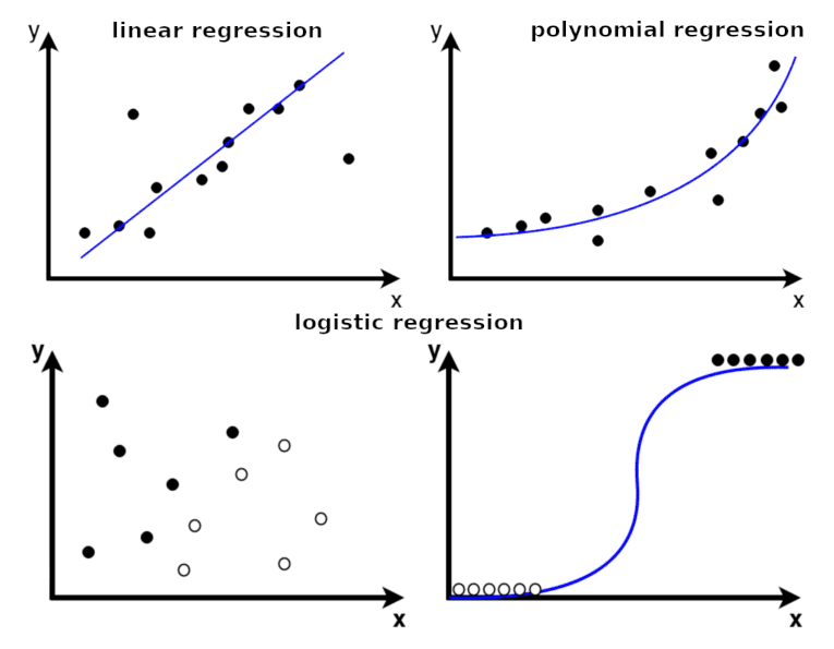
Logistic regression is another important type of regression model, which can be used for classification. Logistic regression takes the predicted value from the linear regression model and sends it to a logistic function which estimates the probability that the instance belongs to a particular class. Logistic regression is the simplest possible neural network consisting of a single artificial neuron.
The main strength of linear regression is its simplicity. The number of parameters in the algorithm is limited, which results in a short training time. Linear regression can be used for simple computer vision tasks where using other algorithms is not ideal, for example, when dealing with very high-dimensional data. In the case of noisy data, linear regression can be improved by methods such as RANdom SAmple Consensus (RANSAC). This algorithm randomly samples data to estimate which samples are outliers that should be ignored, making linear regression more robust.
Support vector machines (SVM)
Support Vector Machines (SVMs) can be used for classification and regression analysis. An SVM algorithm fits a hyperplane, a plane of dimension one less than the dimension of data space, between two classes of data. When drawing a hyperplane, the algorithm tries to maximize the distance to the nearest data points of both classes (the “margin”). The points are called the support vectors, because they “support” the decision boundary.
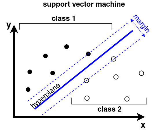
Since most real-life problems are not fully linear, a kernel can be applied to transform the data into higher dimensional space first. A kernel function takes the raw data vectors {X1,X2,...,XN} represented in the original space and returns a dot product of transformed vectors (Xi)⋅(Xj) represented in the higher dimensional space. This is done for all pairs of data i.e. i,j=1,...,N. For computer vision applications, often the radial basis function (RBF) kernel is used. However, when the input to the SVM is histogram-like, a χ2 kernel is preferable.
To enable discrimination between multiple classes, a one-versus-many strategy is usually applied. Here, multiple SVMs are trained, where every SVM discriminates between one class and all others. At test time, the output scores of all SVMs are compared to make a final decision.
The input to an SVM should be a vector that describes the content of an image in a meaningful way. For example, the input can be created with a pipeline consisting of feature detector, feature descriptor and aggregator. An SVM is easy to set up and often gives reasonable results, but the training time can be large if a lot of high-dimensional training samples are available.
Decision trees
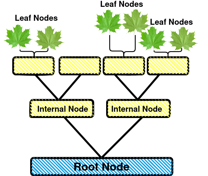
A decision tree is a non-parametric method which predicts a target by learning simple decision rules inferred from the data. These decision-making rules can be represented as a tree structure with nodes. Every node on the tree contains a test (a question), and depending on the outcome, a different branch is followed. This continues until a childless, final leaf is reached. If that is the case, a decision or score is attached to each leaf. During training, at every node the splitting criterion is chosen that results in the best split between the classes. The data is divided over the child nodes according to the criterion. Next, all children are split in similar ways, until pure (one-class) leaves are obtained.
For computer vision algorithms, a decision tree does not generalize very well. The outcome of the classification is sensitive to the precise thresholds in the nodes. Moreover, a decision tree is prone to overfitting, although this can be mitigated by pruning the leaves. On the other hand, a decision tree is perfectly interpretable by humans, which makes it suitable for critical applications.
Random forests
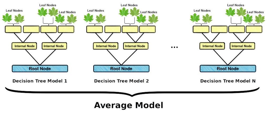
A random forest is a collection of random decision trees. These trees resemble normal decision trees, but the criteria at every node are chosen randomly, out of all possible options. Sometimes, the requirement is relaxed a bit by selecting the best criterion out of a randomly selected subset. While a single random decision tree is very likely to be suboptimal, a collection of these trees in a classifier will offer better results. Indeed, each tree, learning from a subset of data, makes its own unique errors that do not correlate with each other. Thus, these errors disappear when averaging predictions between all models.
A random forest can be trained fast and is fast at inference time. Every separate tree is easy to interpret, which makes a random forest suitable for critical applications. For example, you can use random forest algorithms to remove redundant features, or to find the most relevant features in the input data.
Genetic algorithms
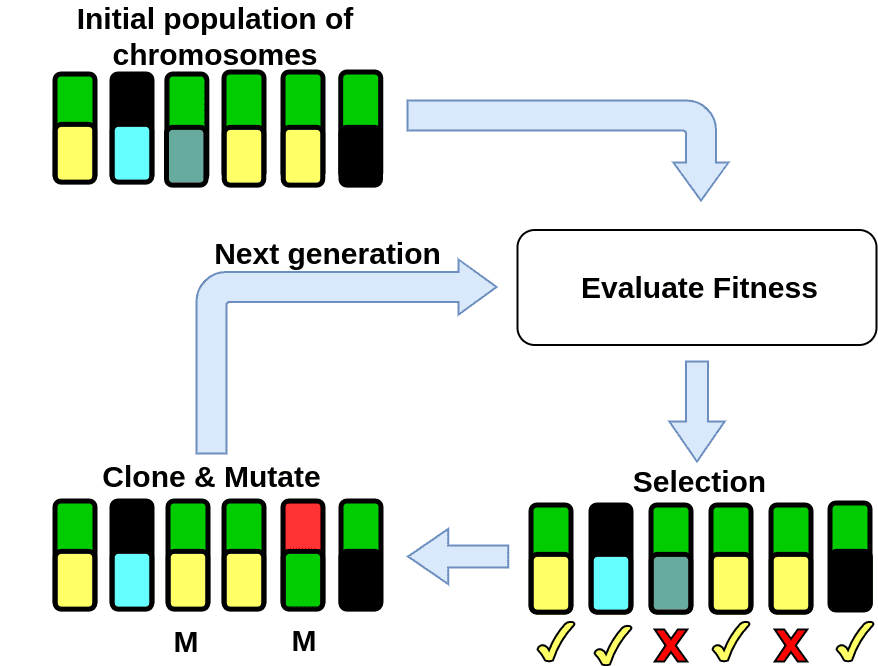
A genetic algorithm is a machine learning method that is inspired by the natural selection process in evolutionary biology. The goal is to find an optimal set of parameters for a model. The algorithm encodes these parameters into a chromosome. At the start of the training process, a population of different chromosomes is initialized (usually randomly) and the fitness value of each chromosome is evaluated. This is the end of a single generation, for the next generation the selected chromosomes are perturbed by mutation (randomly changing some of the values of the chromosomes) and crossover (some parameters of the selected chromosomes are swapped). Then, the fitness value of the perturbed chromosomes can be computed. This process can be repeated for several iterations, which are usually referred to as generations.
For problems with a high number of parameters (e.g. finding weights of neural networks), genetic algorithms tend to require too much computation power before a well performing model is found. Recently, genetic algorithms have been applied to finding optimal hyperparameters for deep learning training. It is reported to result in a better performing model than a model with hyperparameters found through random search.
Which algorithm is right for you?
Traditional machine learning algorithms can be used for a wide range of machine vision applications. The Kapernikov team would love to help you make the best algorithm decision for your project. Do you have a machine vision or automated inspection challenge? Contact us and let’s talk shop with one of our machine vision experts.