Machine learning is a hot topic in research and industry, with new methodologies developed all the time. The speed and complexity of the field makes keeping up with new techniques difficult even for experts — and potentially overwhelming for beginners.
To demystify machine learning and to offer a learning path for those who are new to the core concepts, let’s look at ten different methods, including simple descriptions, visualizations, and examples for each one.
A machine learning algorithm, also called model, is a mathematical expression that represents data in the context of a problem, often a business problem. The aim is to go from data to insight. For example, if an online retailer wants to anticipate sales for the next quarter, they might use a machine learning algorithm that predicts those sales based on past sales and other relevant data. Similarly, a windmill manufacturer might visually monitor important equipment and feed the video data through algorithms trained to identify dangerous cracks.
The ten methods described offer an overview — and a foundation you can build on as you hone your machine learning knowledge and skill:
- Regression
- Classification
- Clustering
- Dimensionality Reduction
- Ensemble Methods
- Neural Nets and Deep Learning
- Transfer Learning
- Reinforcement Learning
- Natural Language Processing
- Word Embeddings
One last thing before we jump in. Let’s distinguish between two general categories of machine learning: supervised and unsupervised. We apply supervised ML techniques when we have a piece of data that we want to predict or explain. We do so by using previous data of inputs and outputs to predict an output based on a new input. For example, you could use supervised ML techniques to help a service business that wants to predict the number of new users who will sign up for the service next month. By contrast, unsupervised ML looks at ways to relate and group data points without the use of a target variable to predict. In other words, it evaluates data in terms of traits and uses the traits to form clusters of items that are similar to one another. For example, you could use unsupervised learning techniques to help a retailer that wants to segment products with similar characteristics — without having to specify in advance which characteristics to use.
Regression
Regression methods fall within the category of supervised ML. They help to predict or explain a particular numerical value based on a set of prior data, for example predicting the price of a property based on previous pricing data for similar properties.
The simplest method is linear regression where we use the mathematical equation of the line (y = m * x + b) to model a data set. We train a linear regression model with many data pairs (x, y) by calculating the position and slope of a line that minimizes the total distance between all of the data points and the line. In other words, we calculate the slope (m) and the y-intercept (b) for a line that best approximates the observations in the data.
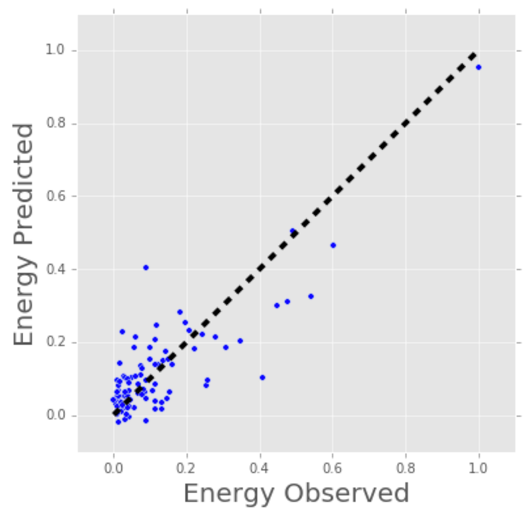
Let’s consider a more a concrete example of linear regression. I once used a linear regression to predict the energy consumption (in kWh) of certain buildings by gathering together the age of the building, number of stories, square feet and the number of plugged wall equipment. Since there were more than one input (age, square feet, etc…), I used a multi-variable linear regression. The principle was the same as a simple one-to-one linear regression, but in this case the “line” I created occurred in multi-dimensional space based on the number of variables.
The plot below shows how well the linear regression model fit the actual energy consumption of building. Now imagine that you have access to the characteristics of a building (age, square feet, etc…) but you don’t know the energy consumption. In this case, we can use the fitted line to approximate the energy consumption of the particular building.
Note that you can also use linear regression to estimate the weight of each factor that contributes to the final prediction of consumed energy. For example, once you have a formula, you can determine whether age, size, or height is most important.
Regression techniques run the gamut from simple (like linear regression) to complex (like regularized linear regression, polynomial regression, decision trees and random forest regressions, neural nets, among others). But don’t get bogged down: start by studying simple linear regression, master the techniques, and move on from there.
Classification
Another class of supervised ML, classification methods predict or explain a class value. For example, they can help predict whether or not an online customer will buy a product. The output can be yes or no: buyer or not buyer. But classification methods aren’t limited to two classes. For example, a classification method could help to assess whether a given image contains a car or a truck. In this case, the output will be 3 different values: 1) the image contains a car, 2) the image contains a truck, or 3) the image contains neither a car nor a truck.
The simplest classification algorithm is logistic regression — which makes it sounds like a regression method, but it’s not. Logistic regression estimates the probability of an occurrence of an event based on one or more inputs.
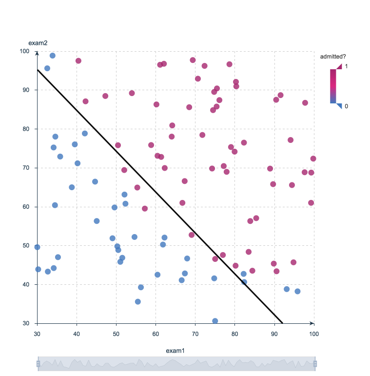
For instance, a logistic regression can take as inputs two exam scores for a student in order to estimate the probability that the student will get admitted to a particular college. Because the estimate is a probability, the output is a number between 0 and 1, where 1 represents complete certainty. For the student, if the estimated probability is greater than 0.5, then we predict that he or she will be admitted. If the estimated probabiliy is less than 0.5, we predict the he or she will be refused.
The chart below plots the scores of previous students along with whether they were admitted. Logistic regression allows us to draw a line that represents the decision boundary.
Because logistic regression is the simplest classification model, it’s a good place to start for classification. As you progress, you can dive into non-linear classifiers such as decision trees, random forests, support vector machines, and neural nets, among others.
Clustering
With clustering methods, we get into the category of unsupervised ML because their goal is to group or cluster observations that have similar characteristics. Clustering methods don’t use output information for training, but instead let the algorithm define the output. In clustering methods, we can only use visualizations to inspect the quality of the solution.
The most popular clustering method is K-Means, where “K” represents the number of clusters that the user chooses to create. (Note that there are various techniques for choosing the value of K, such as the elbow method.)
Roughly, what K-Means does with the data points:
- Randomly chooses K centers within the data.
- Assigns each data point to the closest of the randomly created centers.
- Re-computes the center of each cluster.
- If centers don’t change (or change very little), the process is finished. Otherwise, we return to step 2. (To prevent ending up in an infinite loop if the centers continue to change, set a maximum number of iterations in advance.)
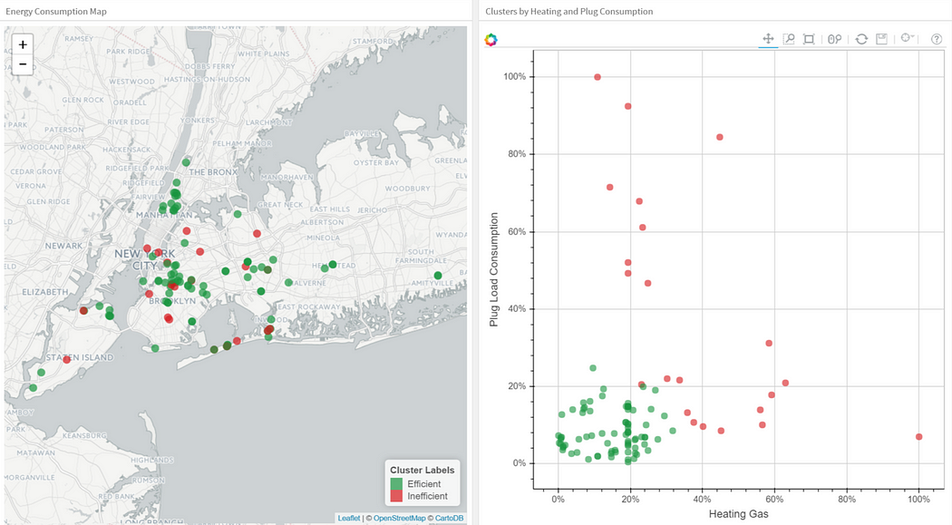
The next plot applies K-Means to a data set of buildings. Each column in the plot indicates the efficiency for each building. The four measurements are related to air conditioning, plugged-in equipment (microwaves, refrigerators, etc…), domestic gas, and heating gas. We chose K=2 for clustering, which makes it easy to interpret one of the clusters as the group of efficient buildings and the other cluster as the group of inefficient buildings. To the left you see the location of the buildings and to right you see two of the four dimensions we used as inputs: plugged-in equipment and heating gas.
As you explore clustering, you’ll encounter very useful algorithms such as Density-Based Spatial Clustering of Applications with Noise (DBSCAN), Mean Shift Clustering, Agglomerative Hierarchical Clustering, Expectation–Maximization Clustering using Gaussian Mixture Models, among others.
Dimensionality Reduction
As the name suggests, we use dimensionality reduction to remove the least important information (sometime redundant columns) from a data set. In practice, I often see data sets with hundreds or even thousands of columns (also called features), so reducing the total number is vital. For instance, images can include thousands of pixels, not all of which matter to your analysis. Or when testing microchips within the manufacturing process, you might have thousands of measurements and tests applied to every chip, many of which provide redundant information. In these cases, you need dimensionality reduction algorithms to make the data set manageable.
The most popular dimensionality reduction method is Principal Component Analysis (PCA), which reduces the dimension of the feature space by finding new vectors that maximize the linear variation of the data. PCA can reduce the dimension of the data dramatically and without losing too much information when the linear correlations of the data are strong. (And in fact you can also measure the actual extent of the information loss and adjust accordingly.)
Another popular method is t-Stochastic Neighbor Embedding (t-SNE), which does non-linear dimensionality reduction. People typically use t-SNE for data visualization, but you can also use it for machine learning tasks like reducing the feature space and clustering, to mention just a few.
The next plot shows an analysis of the MNIST database of handwritten digits. MNIST contains thousands of images of digits from 0 to 9, which researchers use to test their clustering and classification algorithms. Each row of the data set is a vectorized version of the original image (size 28 x 28 = 784) and a label for each image (zero, one, two, three, …, nine). Note that we’re therefore reducing the dimensionality from 784 (pixels) to 2 (dimensions in our visualization). Projecting to two dimensions allows us to visualize the high-dimensional original data set.

Ensemble Methods
Imagine you’ve decided to build a bicycle because you are not feeling happy with the options available in stores and online. You might begin by finding the best of each part you need. Once you assemble all these great parts, the resulting bike will outshine all the other options.
Ensemble methods use this same idea of combining several predictive models (supervised ML) to get higher quality predictions than each of the models could provide on its own. For example, the Random Forest algorithms is an ensemble method that combines many Decision Trees trained with different samples of the data sets. As a result, the quality of the predictions of a Random Forest is higher than the quality of the predictions estimated with a single Decision Tree.
Think of ensemble methods as a way to reduce the variance and bias of a single machine learning model. That’s important because any given model may be accurate under certain conditions but inaccurate under other conditions. With another model, the relative accuracy might be reversed. By combining the two models, the quality of the predictions is balanced out.
The great majority of top winners of Kaggle competitions use ensemble methods of some kind. The most popular ensemble algorithms are Random Forest, XGBoost and LightGBM.
Neural Networks and Deep Learning
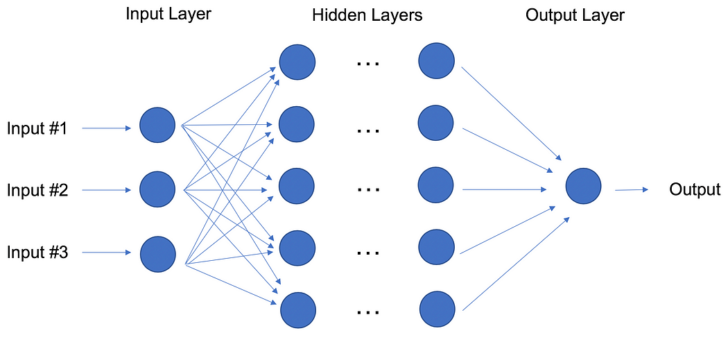
In contrast to linear and logistic regressions which are considered linear models, the objective of neural networks is to capture non-linear patterns in data by adding layers of parameters to the model. In the image below, the simple neural net has three inputs, a single hidden layer with five parameters, and an output layer.
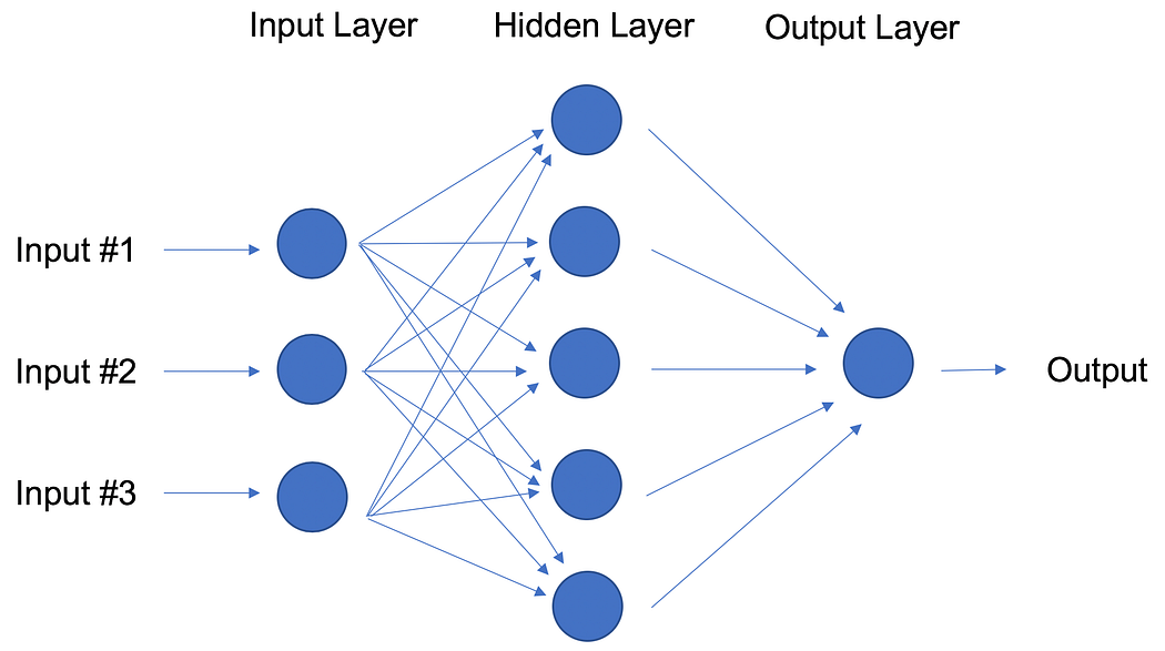
In fact, the structure of neural networks is flexible enough to build our well-known linear and logistic regression. The term Deep learning comes from a neural net with many hidden layers (see next Figure) and encapsulates a wide variety of architectures.
It’s especially difficult to keep up with developments in deep learning, in part because the research and industry communities have doubled down on their deep learning efforts, spawning whole new methodologies every day.
For the best performance, deep learning techniques require a lot of data — and a lot of compute power since the method is self-tuning many parameters within huge architectures. It quickly becomes clear why deep learning practitioners need very powerful computers enhanced with GPUs (graphical processing units).
In particular, deep learning techniques have been extremely successful in the areas of vision (image classification), text, audio and video. The most common software packages for deep learning are Tensorflow and PyTorch.
Transfer Learning
Let’s pretend that you’re a data scientist working in the retail industry. You’ve spent months training a high-quality model to classify images as shirts, t-shirts and polos. Your new task is to build a similar model to classify images of dresses as jeans, cargo, casual, and dress pants. Can you transfer the knowledge built into the first model and apply it to the second model? Yes, you can, using Transfer Learning.
Transfer Learning refers to re-using part of a previously trained neural net and adapting it to a new but similar task. Specifically, once you train a neural net using data for a task, you can transfer a fraction of the trained layers and combine them with a few new layers that you can train using the data of the new task. By adding a few layers, the new neural net can learn and adapt quickly to the new task.
The main advantage of transfer learning is that you need less data to train the neural net, which is particularly important because training for deep learning algorithms is expensive in terms of both time and money (computational resources) — and of course it’s often very difficult to find enough labeled data for the training.
Let’s return to our example and assume that for the shirt model you use a neural net with 20 hidden layers. After running a few experiments, you realize that you can transfer 18 of the shirt model layers and combine them with one new layer of parameters to train on the images of pants. The pants model would therefore have 19 hidden layers. The inputs and outputs of the two tasks are different but the re-usable layers may be summarizing information that is relevant to both, for example aspects of cloth.
Transfer learning has become more and more popular and there are now many solid pre-trained models available for common deep learning tasks like image and text classification.
Reinforcement Learning
Imagine a mouse in a maze trying to find hidden pieces of cheese. The more times we expose the mouse to the maze, the better it gets at finding the cheese. At first, the mouse might move randomly, but after some time, the mouse’s experience helps it realize which actions bring it closer to the cheese.
The process for the mouse mirrors what we do with Reinforcement Learning (RL) to train a system or a game. Generally speaking, RL is a machine learning method that helps an agent learn from experience. By recording actions and using a trial-and-error approach in a set environment, RL can maximize a cumulative reward. In our example, the mouse is the agent and the maze is the environment. The set of possible actions for the mouse are: move front, back, left or right. The reward is the cheese.
You can use RL when you have little to no historical data about a problem, because it doesn’t need information in advance (unlike traditional machine learning methods). In a RL framework, you learn from the data as you go. Not surprisingly, RL is especially successful with games, especially games of “perfect information” like chess and Go. With games, feedback from the agent and the environment comes quickly, allowing the model to learn fast. The downside of RL is that it can take a very long time to train if the problem is complex.
Just as IBM’s Deep Blue beat the best human chess player in 1997, AlphaGo, a RL-based algorithm, beat the best Go player in 2016. The current pioneers of RL are the teams at DeepMind in the UK. More on AlphaGo and DeepMind here.
On April, 2019, the OpenAI Five team was the first AI to beat a world champion team of e-sport Dota 2, a very complex video game that the OpenAI Five team chose because there were no RL algorithms that were able to win it at the time. The same AI team that beat Dota 2’s champion human team also developed a robotic hand that can reorient a block. Read more about the OpenAI Five team here.
You can tell that Reinforcement Learning is an especially powerful form of AI, and we’re sure to see more progress from these teams, but it’s also worth remembering the method’s limitations.
Natural Language Processing
A huge percentage of the world’s data and knowledge is in some form of human language. Can you imagine being able to read and comprehend thousands of books, articles and blogs in seconds? Obviously, computers can’t yet fully understand human text but we can train them to do certain tasks. For example, we can train our phones to autocomplete our text messages or to correct misspelled words. We can even teach a machine to have a simple conversation with a human.
Natural Language Processing (NLP) is not a machine learning method per se, but rather a widely used technique to prepare text for machine learning. Think of tons of text documents in a variety of formats (word, online blogs, ….). Most of these text documents will be full of typos, missing characters and other words that needed to be filtered out. At the moment, the most popular package for processing text is NLTK (Natural Language ToolKit), created by researchers at Stanford.
The simplest way to map text into a numerical representation is to compute the frequency of each word within each text document. Think of a matrix of integers where each row represents a text document and each column represents a word. This matrix representation of the word frequencies is commonly called Term Frequency Matrix (TFM). From there, we can create another popular matrix representation of a text document by dividing each entry on the matrix by a weight of how important each word is within the entire corpus of documents. We call this method Term Frequency Inverse Document Frequency (TFIDF) and it typically works better for machine learning tasks.
Word Embeddings
TFM and TFIDF are numerical representations of text documents that only consider frequency and weighted frequencies to represent text documents. By contrast, word embeddings can capture the context of a word in a document. With the word context, embeddings can quantify the similarity between words, which in turn allows us to do arithmetic with words.
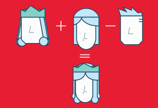
Word2Vec is a method based on neural nets that maps words in a corpus to a numerical vector. We can then use these vectors to find synonyms, perform arithmetic operations with words, or to represent text documents (by taking the mean of all the word vectors in a document). For example, let’s assume that we use a sufficiently big corpus of text documents to estimate word embeddings. Let’s also assume that the words king, queen, man and woman are part of the corpus. Let say that vector(‘word’) is the numerical vector that represents the word ‘word’. To estimate vector(‘woman’), we can perform the arithmetic operation with vectors:
vector(‘king’) + vector(‘woman’) — vector(‘man’) ~ vector(‘queen’)
Word representations allow finding similarities between words by computing the cosine similarity between the vector representation of two words. The cosine similarity measures the angle between two vectors.
We compute word embeddings using machine learning methods, but that’s often a pre-step to applying a machine learning algorithm on top. For instance, suppose we have access to the tweets of several thousand Twitter users. Also suppose that we know which of these Twitter users bought a house. To predict the probability of a new Twitter user buying a house, we can combine Word2Vec with a logistic regression.
You can train word embeddings yourself or get a pre-trained (transfer learning) set of word vectors. To download pre-trained word vectors in 157 different languages, take a look at FastText.
Summary
I’ve tried to cover the ten most important machine learning methods: from the most basic to the bleeding edge. Studying these methods well and fully understanding the basics of each one can serve as a solid starting point for further study of more advanced algorithms and methods.
There is of course plenty of very important information left to cover, including things like quality metrics, cross validation, class imbalance in classification methods, and over-fitting a model, to mention just a few. Stay tuned.
All the visualizations of this blog were done using Watson Studio Desktop.