In machine learning, the term “learning” refers to the process through which machines examine current data and gain new skills and information from it. Machine learning systems employ algorithms to search for patterns in datasets that may include structured data sets, unorganized textual data, numeric data, or even rich media such as audio files, photos, and videos. Machine learning algorithms are computationally expensive, necessitating the need for specialized infrastructure to run at scale.
What is Machine Learning?
Machine learning is a branch of study that aims to train machines to do cognitive tasks in the same way that humans do. While they have far fewer cognitive abilities than the ordinary person, they are capable of quickly processing large amounts of data and extracting significant commercial insights.
Machine learning algorithms employ computational methods to “learn” information directly from data rather than depending on a model based on a preconceived equation. As the number of samples available for learning grows, the algorithms alter their performance. Deep learning is a type of machine learning that is overspecialized.
As a result, as a machine learning practitioner, you may come across a variety of forms of learning, ranging from entire fields of research to individual methodologies.
( Suggested Read- Basics of Machine Learning )
Different Methods of Machine Learning
The main branches of machine learning are listed below. The majority of machine learning algorithms and techniques fall into one of the following groups of methods:
( Related – Types of Machine Learning Methods )
Supervised Learning
The term “Supervised Learning” refers to a scenario in which a model is used to learn a mapping between input samples and the target variable. If you know what you want to teach a machine beforehand, use Supervised Learning.
This usually entails exposing the algorithm to a large amount of training data, allowing the model to study the output, and fine-tuning the parameters until the desired results are obtained. The machine can then be put to the test by allowing it to generate predictions for a “validation data set,” or new data that hasn’t been seen before.
Un-Supervised Learning
Unsupervised learning allows a machine to study a set of data without the assistance of a human. Following the initial exploration, the computer attempts to uncover hidden patterns that link various variables. This method of learning can assist in the classification of data into categories based solely on statistical attributes.
Unsupervised learning does not require big data sets for training, making it significantly faster and easier to implement than supervised learning. Unsupervised learning, in contrast to supervised learning, is based solely on the input data, with no outputs or target variables. As a result, unlike supervised learning, unsupervised learning does not have a teacher correcting the model.
Semi-Supervised Learning
Semi-supervised learning is supervised learning with a small number of labeled instances and a large number of unlabeled examples in the training data.
In contrast to supervised learning, the purpose of a semi-supervised learning model is to make good use of all available data rather than just the labeled data.
Unsupervised and supervised learning techniques are used in semi-supervised learning. Manually categorizing part of the data, for example, can provide an example to the algorithm for how the rest of the data set should be sorted.
Reinforcement learning
Reinforcement learning is a technique that allows a machine to interact with its surroundings. Playing a video game repeatedly and rewarding the algorithm when it does the required action is a simple example. The machine can eventually learn from its experience by repeating the operation thousands or millions of times. The model has some response from which to learn, similar to supervised learning, albeit the feedback may be delayed and statistically noisy, making it difficult for the agent or model to connect cause and effect.
Playing a game in which the player has the objective of earning a high score and can take actions in the game while receiving feedback in the form of punishments or rewards is an example of a reinforcement problem.
Related blog – What is Supervised, Unsupervised, and Reinforcement Learning
Top Machine Learning Techniques
Now Let’s have a look at some of the most popular machine learning techniques that fall under the above-mentioned categories of Machine learning Methods.
Regression
When the output is a real or continuous value, regression techniques are typically employed to generate predictions on numbers. It uses training data to predict new test data since it falls under the category of Supervised Learning. The purpose of regression techniques is to use a previous data set to explain or forecast a certain numerical result. In the case of retail demand forecasting, regression algorithms can use previous pricing data and anticipate the price of a similar property.
Continuous reactions, such as changes in temperature or fluctuations in power consumption, are predicted using regression algorithms. Electricity load forecasting and algorithmic trading are two examples of typical applications.
If you’re working with a data range or the nature of your response is a real number, such as temperature or the time until a piece of equipment fails, use regression techniques.
The simplest and most fundamental method is linear regression. The following equation is used to model a dataset in this case: ( y = m * x + b )
Multiple pairings of data, such as x, y, can be used to train a regression model. To do so, you must first establish a position for the line, as well as its slope, with a minimum distance from all known data points. This is the line that best approximates the data’s observations and can be used to produce predictions for fresh data that hasn’t been seen before.
According to Educuba, Following are some of the most commonly used algorithms in the Regression Technique.
Simple Linear Regression Model
Lasso Regression
Logistic Regression
Support Vector Regression
Multivariate Regression Algorithm
Multiple Regression Algorithm
( Also Read – Working of Linear and Logistic Regression Model )
Classification
A classification model is a Supervised Learning method that generates a conclusion from observed values as one or more categorical outputs. Many AI applications require classification, but it is especially beneficial for eCommerce applications. Classification algorithms, for example, can aid in predicting whether or not a buyer will purchase a product. In this situation, the two classifications are “yes” and “no.” Classification algorithms are not limited to two classes and can be used to categorize materials into many different groups. The Classification model employs a variety of methods, including Logistic Regression, Multilayer Perception, and others. In this model, we classify our data into distinct categories and assign labels to those categories. There are two types of classifiers:
Classifiers with two unique classifications and two outputs are known as Binary classifiers.
Classifiers having more than two classes are known as Multi-class classifiers.
Clustering
Clustering is a Machine Learning approach for categorizing data points into distinct groups. If we have a set of objects or data points, we can use a clustering method to analyze and group them based on their traits and characteristics. Because of its statistical approaches, this unsupervised procedure is applied. Cluster algorithms use training data to make predictions and form groups based on resemblance or unfamiliarity.
( Related – Applications of Clustering )
Unsupervised learning approaches include clustering algorithms. K-means clustering, mean-shift, and expectation-maximization are three popular clustering techniques. They categorize data points into groups based on features that are similar or shared.
When huge amounts of data need to be segmented or categorized, grouping or clustering techniques are very effective in business applications.
Some of the Clustering Methods are given below-
Density-based methods
Hierarchical methods.
Partitioning methods
Grid-based methods
( Read further on this – Types of Clustering Algorithm )
Decision Tree
It’s a supervised learning algorithm that’s commonly used to solve classification difficulties. It works for both categorical and continuous dependent variables, which is surprising. We divide the population into two or more homogenous sets using this approach. This is done to create as many separate groups as feasible based on the most important attributes/independent variables.
According to MobiDev, The Decision tree algorithm categorizes objects by responding to “questions” regarding their qualities at nodal points. One of the branches is chosen based on the answer, and another question is presented at the next junction until the algorithm reaches the tree’s “leaf,” which represents the ultimate answer.
Knowledge management platforms for customer service, predictive pricing, and product planning are examples of decision tree applications.
( Also Read – Decision Tree in Machine Learning )
Neural Networks
Neural networks are designed to resemble the brain’s structure: each artificial neuron connects to many other neurons, and millions of neurons work together to form a sophisticated cognitive structure. The structure of neural networks is multilayer: neurons in one layer transfer data to many neurons in the next layer, and so on.
The data eventually reaches the output layer, when the network decides how to deal with a problem, categorize an object, and so on. The study of neural networks is characterized as “deep learning” because of its multi-layer structure.
Neural networks can be used for machine translation, fraud detection, and virtual assistant services in the telecoms and media industries. They’re used in the financial industry to detect fraud, manage portfolios, and assess risk.
( Related – Applications of Neural Networks )
Anomaly Detection
The process of recognizing unexpected items or events in a data set is known as anomaly detection. Detection of fraud, failure detection, computer health monitoring, and more applications employ this technology. Anomaly detection can be divided into three categories:
Point anomalies: When a single piece of data is unexpected, this is referred to as a point anomaly.
Contextual anomalies: Contextual anomalies are anomalies that are context-specific.
Collective anomalies: When a group or collection of linked data elements is anomalous, it is referred to as a collective anomaly.
Google’s self-driving cars and robots get a lot of press, but the company’s real future is in machine learning, the technology that enables computers to get smarter and more personal.– Eric Schmidt (Google Chairman)
We are probably living in the most defining period of human history. The period when computing moved from large mainframes to PCs to the cloud. But what makes it defining is not what has happened but what is coming our way in years to come. What makes this period exciting and enthralling for someone like me is the democratization of the various tools, techniques, and machine learning algorithms that followed the boost in computing. Welcome to the world of data science!
Today, as a data scientist, I can build data-crunching machines with complex algorithms for a few dollars per hour. But reaching here wasn’t easy! I had my dark days and nights.
Learning Objectives
Major focus on commonly used machine learning techniques and algorithms.
Algorithms covered – Linear regression, logistic regression, Naive Bayes, kNN, Random forest, etc.
Learn both theory and implementation of the machine learning algorithms in R and python.
Are you a beginner looking for a place to start your data science journey and learn machine learning models? Presenting a list of comprehensive courses, full of knowledge and data science learning, curated just for you to learn data science (using Python) from scratch:
Machine Learning Certification Course for Beginners
Introduction to Data Science
Certified AI & ML Blackbelt+ Program
Table of Contents
Who Can Benefit the Most From This Guide?
3 Types Of Machine Learning Algorithms
List of Common Machine Learning Algorithms
Gradient Boosting Algorithms
Practice Problems
Conclusion
Who Can Benefit the Most From This Guide?
What I am giving out today is probably the most valuable guide I have ever created.
The idea behind creating this guide is to simplify the journey of aspiring data scientists and machine learning (which is part of artificial intelligence) enthusiasts across the world. Through this guide, I will enable you to work on machine-learning problems and gain from experience. I am providing a high-level understanding of various machine learning algorithms along with R & Python codes to run them. These should be sufficient to get your hands dirty. You can also check out our Machine Learning Course.
Essentials of machine learning algorithms with implementation in R and Python
I have deliberately skipped the statistics behind these techniques and artificial neural networks, as you don’t need to understand them initially. So, if you are looking for a statistical understanding of these algorithms, you should look elsewhere. But, if you want to equip yourself to start building a machine learning project, you are in for a treat.
3 Types of Machine Learning Algorithms
Supervised Learning Algorithms
How it works: This algorithm consists of a target/outcome variable (or dependent variable) which is to be predicted from a given set of predictors (independent variables). Using this set of variables, we generate a function that maps input data to desired outputs. The training process continues until the model achieves the desired level of accuracy on the training data. Examples of Supervised Learning: Regression, Decision Tree, Random Forest, KNN, Logistic Regression, etc.
Unsupervised Learning Algorithms
How it works: In this algorithm, we do not have any target or outcome variable to predict / estimate (which is called unlabelled data). It is used for recommendation systems or clustering populations in different groups. clustering algorithms are widely used for segmenting customers into different groups for specific interventions. Examples of Unsupervised Learning: Apriori algorithm, K-means clustering.
Reinforcement Learning Algorithms
How it works: Using this algorithm, the machine is trained to make specific decisions. The machine is exposed to an environment where it trains itself continually using trial and error. This machine learns from past experience and tries to capture the best possible knowledge to make accurate business decisions. Example of Reinforcement Learning: Markov Decision Process
List of Top 10 Common Machine Learning Algorithms
Here is the list of commonly used machine learning algorithms. These algorithms can be applied to almost any data problem:
Linear Regression
Logistic Regression
Decision Tree
SVM
Naive Bayes
kNN
K-Means
Random Forest
Dimensionality Reduction Algorithms
Gradient Boosting algorithms
GBM
XGBoost
LightGBM
CatBoost
Linear Regression
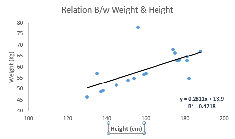
It is used to estimate real values (cost of houses, number of calls, total sales, etc.) based on a continuous variable(s). Here, we establish the relationship between independent and dependent variables by fitting the best line. This best-fit line is known as the regression line and is represented by a linear equation Y= a*X + b.
The best way to understand linear regression is to relive this experience of childhood. Let us say you ask a child in fifth grade to arrange people in his class by increasing the order of weight without asking them their weights! What do you think the child will do? He/she would likely look (visually analyze) at the height and build of people and arrange them using a combination of these visible parameters. This is linear regression in real life! The child has actually figured out that height and build would be correlated to weight by a relationship, which looks like the equation above.
In this equation:
Y – Dependent Variable
a – Slope
X – Independent variable
b – Intercept
These coefficients a and b are derived based on minimizing the sum of the squared difference of distance between data points and the regression line.
Look at the below example. Here we have identified the best-fit line having linear equation y=0.2811x+13.9. Now using this equation, we can find the weight, knowing the height of a person.
Linear Regression is mainly of two types: Simple Linear Regression and Multiple Linear Regression. Simple Linear Regression is characterized by one independent variable. And, Multiple Linear Regression(as the name suggests) is characterized by multiple (more than 1) independent variables. While finding the best-fit line, you can fit a polynomial or curvilinear regression. And these are known as polynomial or curvilinear regression.
Here’s a coding window to try out your hand and build your own linear regression model in Python:
R Code:
#Load Train and Test datasets
#Identify feature and response variable(s) and values must be numeric and numpy arrays
x_train <- input_variables_values_training_datasets
y_train <- target_variables_values_training_datasets
x_test <- input_variables_values_test_datasets
x <- cbind(x_train,y_train)
# Train the model using the training sets and check score
linear <- lm(y_train ~ ., data = x)
summary(linear)
#Predict Output
predicted= predict(linear,x_test)
Logistic Regression
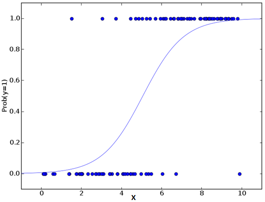
Don’t get confused by its name! It is a classification algorithm, not a regression algorithm. It is used to estimate discrete values ( Binary values like 0/1, yes/no, true/false ) based on a given set of independent variable(s). In simple words, it predicts the probability of the occurrence of an event by fitting data to a logistic function. Hence, it is also known as logit regression. Since it predicts the probability, its output values lie between 0 and 1 (as expected).
Again, let us try and understand this through a simple example.
Let’s say your friend gives you a puzzle to solve. There are only 2 outcome scenarios – either you solve it, or you don’t. Now imagine that you are being given a wide range of puzzles/quizzes in an attempt to understand which subjects you are good at. The outcome of this study would be something like this – if you are given a trigonometry-based tenth-grade problem, you are 70% likely to solve it. On the other hand, if it is a grade fifth history question, the probability of getting an answer is only 30%. This is what Logistic Regression provides you.
Coming to the math, the log odds of the outcome are modeled as a linear combination of the predictor variables.
odds= p/ (1-p) = probability of event occurrence / probability of not event occurrence
ln(odds) = ln(p/(1-p))
logit(p) = ln(p/(1-p)) = b0+b1X1+b2X2+b3X3....+bkXk
Above, p is the probability of the presence of the characteristic of interest. It chooses parameters that maximize the likelihood of observing the sample values rather than that minimize the sum of squared errors (like in ordinary regression).
Now, you may ask, why take a log? For the sake of simplicity, let’s just say that this is one of the best mathematical ways to replicate a step function. I can go into more details, but that will beat the purpose of this article.
Build your own logistic regression model in Python here and check the accuracy:
R Code:
x <- cbind(x_train,y_train)
# Train the model using the training sets and check score
logistic <- glm(y_train ~ ., data = x,family='binomial')
summary(logistic)
#Predict Output
predicted= predict(logistic,x_test)
Furthermore…
There are many different steps that could be tried in order to improve the model:
including interaction terms
removing features
regularization techniques
using a non-linear model
Decision Tree
This is one of my favorite algorithms, and I use it quite frequently. It is a type of supervised learning algorithm that is mostly used for classification problems. Surprisingly, it works for both categorical and continuous dependent variables. In this algorithm, we split the population into two or more homogeneous sets. This is done based on the most significant attributes/ independent variables to make as distinct groups as possible. For more details, you can read Decision Tree Simplified.
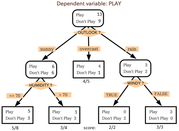
Source: statsexchange
In the image above, you can see that population is classified into four different groups based on multiple attributes to identify ‘if they will play or not’. To split the population into different heterogeneous groups, it uses various techniques like Gini, Information Gain, Chi-square, and entropy.
The best way to understand how the decision tree works, is to play Jezzball – a classic game from Microsoft (image below). Essentially, you have a room with moving walls and you need to create walls such that the maximum area gets cleared off without the balls.
So, every time you split the room with a wall, you are trying to create 2 different populations within the same room. Decision trees work in a very similar fashion by dividing a population into as different groups as possible.
More: Simplified Version of Decision Tree Algorithms
Let’s get our hands dirty and code our own decision tree in Python!
R Code:
library(rpart)
x <- cbind(x_train,y_train)
# grow tree
fit <- rpart(y_train ~ ., data = x,method="class")
summary(fit)
#Predict Output
predicted= predict(fit,x_test)
SVM (Support Vector Machine)
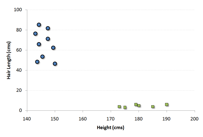
It is a classification method. In this algorithm, we plot each data item as a point in n-dimensional space (where n is the number of features you have), with the value of each feature being the value of a particular coordinate.
For example, if we only had two features like the Height and Hair length of an individual, we’d first plot these two variables in two-dimensional space where each point has two coordinates (these co-ordinates are known as Support Vectors)
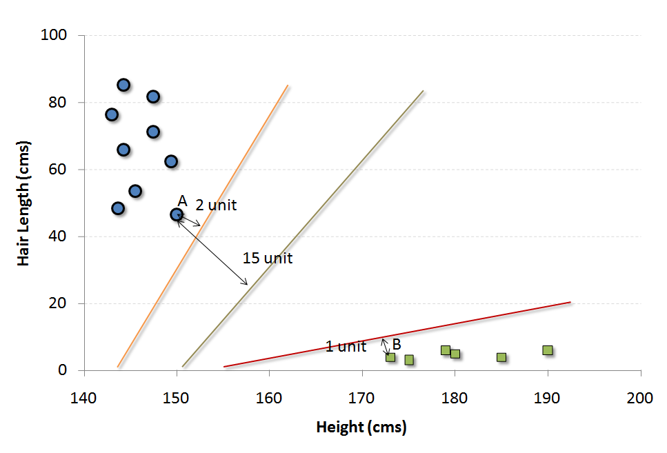
Now, we will find some lines that split the data between the two differently classified groups of data. This will be the line such that the distances from the closest point in each of the two groups will be the farthest away. If there are more variables, a hyperplane is used to separate the classes.
In the example shown above, the line which splits the data into two differently classified groups is the blackline since the two closest points are the farthest apart from the line. This line is our classifier. Then, depending on where the testing data lands on either side of the line, that’s what class we can classify the new data as.
More: Simplified Version of Support Vector Machine Think of this algorithm as playing JezzBall in n-dimensional space. The tweaks in the game are:
You can draw lines/planes at any angle (rather than just horizontal or vertical as in the classic game)
The objective of the game is to segregate balls of different colors in different rooms.
And the balls are not moving.
Try your hand and design an SVM model in Python through this coding window:
R Code:
library(e1071)
x <- cbind(x_train,y_train)
# Fitting model
fit <-svm(y_train ~ ., data = x)
summary(fit)
#Predict Output
predicted= predict(fit,x_test)
Naive Bayes
It is a classification technique based on Bayes’ theorem with an assumption of independence between predictors. In simple terms, a Naive Bayes classifier assumes that the presence of a particular feature in a class is unrelated to the presence of any other feature. For example, a fruit may be considered to be an apple if it is red, round, and about 3 inches in diameter. Even if these features depend on each other or upon the existence of the other features, a naive Bayes classifier would consider all of these properties to independently contribute to the probability that this fruit is an apple.
The Naive Bayesian model is easy to build and particularly useful for very large data sets. Along with simplicity, Naive Bayes is known to outperform even highly sophisticated classification methods.
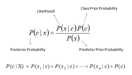
Bayes theorem provides a way of calculating posterior probability P(c|x) from P(c), P(x), and P(x|c). Look at the equation below:
Here,
P(c|x) is the posterior probability of class (target) given predictor (attribute).
P(c) is the prior probability of the class.
P(x|c) is the likelihood which is the probability of the predictor given the class.
P(x) is the prior probability of the predictor.
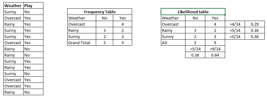
Example: Let’s understand it using an example. Below is a training data set of weather and the corresponding target variable, ‘Play.’ Now, we need to classify whether players will play or not based on weather conditions. Let’s follow the below steps to perform it.
Step 1: Convert the data set to a frequency table.
Step 2: Create a Likelihood table by finding the probabilities like Overcast probability = 0.29 and probability of playing is 0.64.
Step 3: Now, use the Naive Bayesian equation to calculate the posterior probability for each class. The class with the highest posterior probability is the outcome of the prediction.
Problem: Players will pay if the weather is sunny. Is this statement correct?
We can solve it using above discussed method, so P(Yes | Sunny) = P( Sunny | Yes) * P(Yes) / P (Sunny)
Here we have P (Sunny | Yes) = 3/9 = 0.33, P(Sunny) = 5/14 = 0.36, P(Yes)= 9/14 = 0.64
Now, P (Yes | Sunny) = 0.33 * 0.64 / 0.36 = 0.60, which has a higher probability.
Naive Bayes uses a similar method to predict the probability of different classes based on various attributes. This algorithm is mostly used in text classification and with problems having multiple classes.
Code for a Naive Bayes classification model in Python:
R Code:
library(e1071)
x <- cbind(x_train,y_train)
# Fitting model
fit <-naiveBayes(y_train ~ ., data = x)
summary(fit)
#Predict Output
predicted= predict(fit,x_test)
kNN (k- Nearest Neighbors)
It can be used for both classification and regression problems. However, it is more widely used in classification problems in the industry. K nearest neighbors is a simple algorithm that stores all available cases and classifies new cases by a majority vote of its k neighbors. The case assigned to the class is most common amongst its K nearest neighbors measured by a distance function.
These distance functions can be Euclidean, Manhattan, Minkowski, and Hamming distances. The first three functions are used for continuous functions, and the fourth one (Hamming) for categorical variables. If K = 1, then the case is simply assigned to the class of its nearest neighbor. At times, choosing K turns out to be a challenge while performing kNN modeling.
More: Introduction to k-nearest neighbors: Simplified.
KNN can easily be mapped to our real lives. If you want to learn about a person with whom you have no information, you might like to find out about his close friends and the circles he moves in and gain access to his/her information!
Things to consider before selecting kNN:
KNN is computationally expensive
Variables should be normalized else higher range variables can bias it
Works on pre-processing stage more before going for kNN like an outlier, noise removal
Python Code:
R Code:
library(knn)
x <- cbind(x_train,y_train)
# Fitting model
fit <-knn(y_train ~ ., data = x,k=5)
summary(fit)
#Predict Output
predicted= predict(fit,x_test)
K-Means
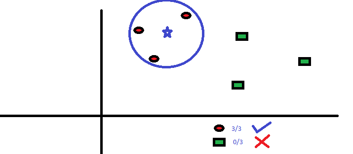
It is a type of unsupervised algorithm which solves the clustering problem. Its procedure follows a simple and easy way to classify a given data set through a certain number of clusters (assume k clusters). Data points inside a cluster are homogeneous and heterogeneous to peer groups.
Remember figuring out shapes from ink blots? k means is somewhat similar to this activity. You look at the shape and spread to decipher how many different clusters/populations are present!
How K-means forms cluster:
K-means picks k number of points for each cluster known as centroids.
Each data point forms a cluster with the closest centroids, i.e., k clusters.
Finds the centroid of each cluster based on existing cluster members. Here we have new centroids.
As we have new centroids, repeat steps 2 and 3. Find the closest distance for each data point from new centroids and get associated with new k-clusters. Repeat this process until convergence occurs, i.e., centroids do not change.
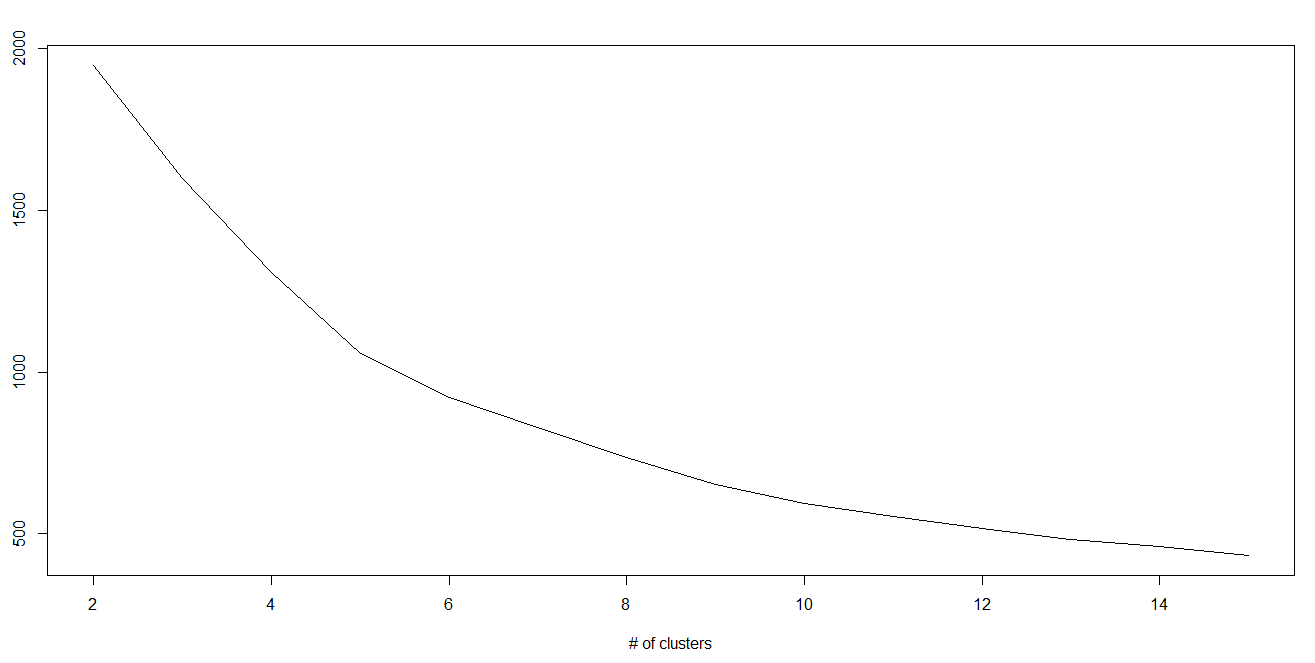
How to determine the value of K:
In K-means, we have clusters, and each cluster has its own centroid. The sum of the square of the difference between the centroid and the data points within a cluster constitutes the sum of the square value for that cluster. Also, when the sum of square values for all the clusters is added, it becomes a total within the sum of the square value for the cluster solution.
We know that as the number of clusters increases, this value keeps on decreasing, but if you plot the result, you may see that the sum of squared distance decreases sharply up to some value of k and then much more slowly after that. Here, we can find the optimum number of clusters.
Python Code:
R Code:
library(cluster)
fit <- kmeans(X, 3) # 5 cluster solution
Random Forest
Random Forest is a trademarked term for an ensemble learning of decision trees. In Random Forest, we’ve got a collection of decision trees (also known as “Forest”). To classify a new object based on attributes, each tree gives a classification, and we say the tree “votes” for that class. The forest chooses the classification having the most votes (over all the trees in the forest).
Each tree is planted & grown as follows:
If the number of cases in the training set is N, then a sample of N cases is taken at random but with replacement. This sample will be the training set for growing the tree.
If there are M input variables, a number m<<M is specified such that at each node, m variables are selected at random out of the M, and the best split on this m is used to split the node. The value of m is held constant during the forest growth.
Each tree is grown to the largest extent possible. There is no pruning.
For more details on this algorithm, compared with the decision tree and tuning model parameters, I would suggest you read these articles:
Introduction to Random forest – Simplified
Comparing a CART model to Random Forest (Part 1)
Comparing a Random Forest to a CART model (Part 2)
Tuning the parameters of your Random Forest model
Python Code:
R Code:
library(randomForest)
x <- cbind(x_train,y_train)
# Fitting model
fit <- randomForest(Species ~ ., x,ntree=500)
summary(fit)
#Predict Output
predicted= predict(fit,x_test)
Dimensionality Reduction Algorithms
In the last 4-5 years, there has been an exponential increase in data capturing at every possible stage. Corporates/ Government Agencies/ Research organizations are not only coming up with new sources, but also they are capturing data in great detail.
For example, E-commerce companies are capturing more details about customers like their demographics, web crawling history, what they like or dislike, purchase history, feedback, and many others to give them personalized attention more than your nearest grocery shopkeeper.
As data scientists, the data we are offered also consists of many features, this sounds good for building a good robust model, but there is a challenge. How’d you identify highly significant variable(s) out of 1000 or 2000? In such cases, the dimensionality reduction algorithm helps us, along with various other algorithms like Decision Tree, Random Forest, PCA (principal component analysis), Factor Analysis, Identity-based on the correlation matrix, missing value ratio, and others.
To know more about these algorithms, you can read “Beginners Guide To Learn Dimension Reduction Techniques“.
Now, let’s look at the 4 most commonly used gradient boosting algorithms.
GBM
GBM is a boosting algorithm used when we deal with plenty of data to make a prediction with high prediction power. Boosting is actually an ensemble of learning algorithms that combines the prediction of several base estimators in order to improve robustness over a single estimator. It combines multiple weak or average predictors to build a strong predictor. These boosting algorithms always work well in data science competitions like Kaggle, AV Hackathon, and CrowdAnalytix.
More: Know about Boosting algorithms in detail Python Code:
R Code:
library(caret)
x <- cbind(x_train,y_train)
# Fitting model
fitControl <- trainControl( method = "repeatedcv", number = 4, repeats = 4)
fit <- train(y ~ ., data = x, method = "gbm", trControl = fitControl,verbose = FALSE)
predicted= predict(fit,x_test,type= "prob")[,2]
GradientBoostingClassifier and Random Forest are two different boosting tree classifiers, and often people ask about the difference between these two algorithms.
XGBoost
Another classic gradient-boosting algorithm that’s known to be the decisive choice between winning and losing in some Kaggle competitions is the XGBoost. It has an immensely high predictive power, making it the best choice for accuracy in events. It possesses both a linear model and the tree learning algorithm, making the algorithm almost 10x faster than existing gradient booster techniques.
One of the most interesting things about the XGBoost is that it is also called a regularized boosting technique. This helps to reduce overfit modeling and has massive support for a range of languages such as Scala, Java, R, Python, Julia, and C++.
The support includes various objective functions, including regression, classification, and ranking. Supports distributed and widespread training on many machines that encompass GCE, AWS, Azure, and Yarn clusters. XGBoost can also be integrated with Spark, Flink, and other cloud dataflow systems with built-in cross-validation at each iteration of the boosting process.
Python Code:
R Code:
require(caret)

x <- cbind(x_train,y_train)

# Fitting model

TrainControl <- trainControl( method = "repeatedcv", number = 10, repeats = 4)

model<- train(y ~ ., data = x, method = "xgbLinear", trControl = TrainControl,verbose = FALSE)

OR

model<- train(y ~ ., data = x, method = "xgbTree", trControl = TrainControl,verbose = FALSE)

predicted <- predict(model, x_test)
LightGBM
LightGBM is a gradient-boosting framework that uses tree-based learning algorithms. It is designed to be distributed and efficient with the following advantages:
Faster training speed and higher efficiency
Lower memory usage
Better accuracy
Parallel and GPU learning supported
Capable of handling large-scale data
The framework is a fast and high-performance gradient-boosting one based on decision tree algorithms used for ranking, classification, and many other machine-learning tasks. It was developed under the Distributed Machine Learning Toolkit Project of Microsoft.
Since the LightGBM is based on decision tree algorithms, it splits the tree leaf-wise with the best fit, whereas other boosting algorithms split the tree depth-wise or level-wise rather than leaf-wise. So when growing on the same leaf node in Light GBM, the leaf-wise algorithm can reduce more loss than the level-wise algorithm, resulting in much better accuracy, which any existing boosting algorithms can rarely achieve.
Also, it is surprisingly very fast, hence the word ‘Light.’
Python Code:
data = np.random.rand(500, 10) # 500 entities, each contains 10 features
label = np.random.randint(2, size=500) # binary target

train_data = lgb.Dataset(data, label=label)
test_data = train_data.create_valid('test.svm')

param = {'num_leaves':31, 'num_trees':100, 'objective':'binary'}
param['metric'] = 'auc'

num_round = 10
bst = lgb.train(param, train_data, num_round, valid_sets=[test_data])

bst.save_model('model.txt')

# 7 entities, each contains 10 features
data = np.random.rand(7, 10)
ypred = bst.predict(data)
R Code:
library(RLightGBM)
data(example.binary)
#Parameters

num_iterations <- 100
config <- list(objective = "binary",  metric="binary_logloss,auc", learning_rate = 0.1, num_leaves = 63, tree_learner = "serial", feature_fraction = 0.8, bagging_freq = 5, bagging_fraction = 0.8, min_data_in_leaf = 50, min_sum_hessian_in_leaf = 5.0)

#Create data handle and booster
handle.data <- lgbm.data.create(x)

lgbm.data.setField(handle.data, "label", y)

handle.booster <- lgbm.booster.create(handle.data, lapply(config, as.character))

#Train for num_iterations iterations and eval every 5 steps

lgbm.booster.train(handle.booster, num_iterations, 5)

#Predict
pred <- lgbm.booster.predict(handle.booster, x.test)

#Test accuracy
sum(y.test == (y.pred > 0.5)) / length(y.test)

#Save model (can be loaded again via lgbm.booster.load(filename))
lgbm.booster.save(handle.booster, filename = "/tmp/model.txt")
If you’re familiar with the Caret package in R, this is another way of implementing the LightGBM.
require(caret)
require(RLightGBM)
data(iris)

model <-caretModel.LGBM()

fit <- train(Species ~ ., data = iris, method=model, verbosity = 0)
print(fit)
y.pred <- predict(fit, iris[,1:4])

library(Matrix)
model.sparse <- caretModel.LGBM.sparse()

#Generate a sparse matrix
mat <- Matrix(as.matrix(iris[,1:4]), sparse = T)
fit <- train(data.frame(idx = 1:nrow(iris)), iris$Species, method = model.sparse, matrix = mat, verbosity = 0)
print(fit)
Catboost
CatBoost is one of open-sourced machine learning algorithms from Yandex. It can easily integrate with deep learning frameworks like Google’s TensorFlow and Apple’s Core ML. The best part about CatBoost is that it does not require extensive data training like other ML models and can work on a variety of data formats, not undermining how robust it can be.
Catboost can automatically deal with categorical variables without showing the type conversion error, which helps you to focus on tuning your model better rather than sorting out trivial errors. Make sure you handle missing data well before you proceed with the implementation.
Python Code:
import pandas as pd
import numpy as np

from catboost import CatBoostRegressor

#Read training and testing files
train = pd.read_csv("train.csv")
test = pd.read_csv("test.csv")

#Imputing missing values for both train and test
train.fillna(-999, inplace=True)
test.fillna(-999,inplace=True)

#Creating a training set for modeling and validation set to check model performance
X = train.drop(['Item_Outlet_Sales'], axis=1)
y = train.Item_Outlet_Sales

from sklearn.model_selection import train_test_split

X_train, X_validation, y_train, y_validation = train_test_split(X, y, train_size=0.7, random_state=1234)
categorical_features_indices = np.where(X.dtypes != np.float)[0]

#importing library and building model
from catboost import CatBoostRegressormodel=CatBoostRegressor(iterations=50, depth=3, learning_rate=0.1, loss_function='RMSE')

model.fit(X_train, y_train,cat_features=categorical_features_indices,eval_set=(X_validation, y_validation),plot=True)

submission = pd.DataFrame()

submission['Item_Identifier'] = test['Item_Identifier']
submission['Outlet_Identifier'] = test['Outlet_Identifier']
submission['Item_Outlet_Sales'] = model.predict(test)
Now, it’s time to take the plunge and actually play with some other real-world datasets. So are you ready to take on the challenge? Accelerate your data science journey with the following practice problems:
Conclusion
By now, I am sure you would have an idea of commonly used machine learning algorithms. My sole intention behind writing this article and providing the codes in R and Python is to get you started right away. If you are keen to master machine learning algorithms, start right away. Take up problems, develop a physical understanding of the process, apply these codes, and watch the fun!
Key Takeaways
We are now familiar with some of the most common ML algorithms used in the industry.
We’ve covered the advantages and disadvantages of various ML algorithms.
We’ve also learned the basic implementation details in R and Python languages.
Frequently Asked Questions
Q1. Which algorithm is mostly used in machine learning?
A. While the suitable algorithm depends on the problem, gradient-boosted decision trees are mostly used to balance performance and interpretability.
Q2. What is the difference between supervised and unsupervised ML?
A. In the supervised learning model, the labels associated with the features are given. In unsupervised learning, no labels are provided for the model.
Q3. What are the main 3 types of ML models?
A. The 3 main types of ML models are based on Supervised Learning, Unsupervised Learning, and Reinforcement Learning.

