Category: Classification in Machine Learning: An Introduction

Nowadays, many industries have been dealing with very large data sets of different types. Manually processing all that information can be time-consuming and might not even add value in the long term. Many strategies, from simple automation to machine learning techniques, are being applied for a better return on investment. This conceptual blog will cover one of the most important concepts; classification in machine learning. 

We will start by defining what classification is in Machine Learning before clarifying the two types of learners in machine learning and the difference between classification and regression. Then, we will cover some real-world scenarios where classification can be used. After that, we will introduce all the different types of classification and deep dive into some examples of classification algorithms. Finally, we will provide hands-on practice on the implementation of a few algorithms. 

What is Classification in Machine Learning?

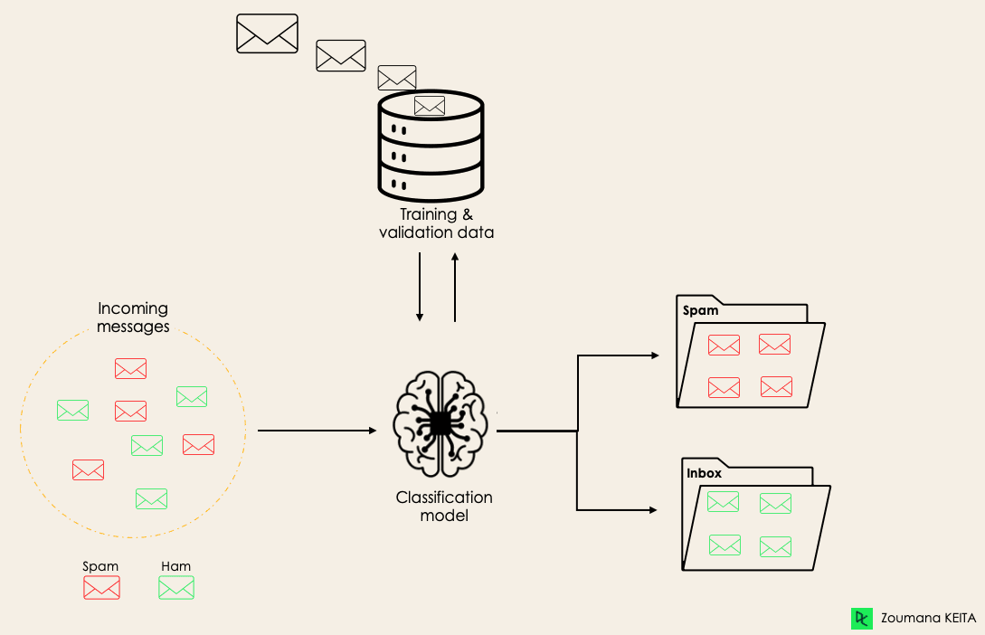
Classification is a supervised machine learning method where the model tries to predict the correct label of a given input data. In classification, the model is fully trained using the training data, and then it is evaluated on test data before being used to perform prediction on new unseen data.

For instance, an algorithm can learn to predict whether a given email is spam or ham (no spam), as illustrated below. 

Before diving into the classification concept, we will first understand the difference between the two types of learners in classification: lazy and eager learners. Then we will clarify the misconception between classification and regression. 

Lazy Learners Vs. Eager Learners

There are two types of learners in machine learning classification: lazy and eager learners. 

Eager learners are machine learning algorithms that first build a model from the training dataset before making any prediction on future datasets. They spend more time during the training process because of their eagerness to have a better generalization during the training from learning the weights, but they require less time to make predictions. 

Most machine learning algorithms are eager learners, and below are some examples: 

• Logistic Regression. 
• Support Vector Machine. 
• Decision Trees. 
• Artificial Neural Networks. 

Lazy learners or instance-based learners, on the other hand, do not create any model immediately from the training data, and this is where the lazy aspect comes from. They just memorize the training data, and each time there is a need to make a prediction, they search for the nearest neighbor from the whole training data, which makes them very slow during prediction. Some examples of this kind are: 

• K-Nearest Neighbor. 
• Case-based reasoning. 

However, some algorithms, such as BallTrees and KDTrees, can be used to improve the prediction latency. 

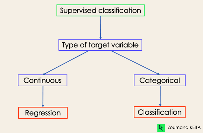
Machine Learning Classification Vs. Regression

There are four main categories of Machine Learning algorithms: supervised, unsupervised, semi-supervised, and reinforcement learning. 

Even though classification and regression are both from the category of supervised learning, they are not the same. 

• The prediction task is a classification when the target variable is discrete. An application is the identification of the underlying sentiment of a piece of text. 
• The prediction task is a regression when the target variable is continuous. An example can be the prediction of the salary of a person given their education degree, previous work experience, geographical location, and level of seniority.

If you are interested in knowing more about classification, courses on Supervised Learning with scikit-learn  and Supervised Learning in R might be helpful. They provide you with a better understanding of how each algorithm approaches tasks and the Python and R functions required to implement them. 

Regarding regression, Introduction to Regression in R and Introduction to Regression with statsmodels in Python will help you explore different types of regression models as well as their implementation in R and Python.

Examples of Machine Learning Classification in Real Life 

Supervised Machine Learning Classification has different applications in multiple domains of our day-to-day life. Below are some examples. 

Healthcare 

Training a machine learning model on historical patient data can help healthcare specialists accurately analyze their diagnoses:

• During the COVID-19 pandemic, machine learning models were implemented to efficiently predict whether a person had COVID-19 or not. 
• Researchers can use machine learning models to predict new diseases that are more likely to emerge in the future. 

Education 

Education is one of the domains dealing with the most textual, video, and audio data. This unstructured information can be analyzed with the help of Natural Language technologies to perform different tasks such as:

• The classification of documents per category. 
• Automatic identification of the underlying language of students’ documents during their application. 
• Analysis of students’ feedback sentiments about a Professor.  

Transportation

Transportation is the key component of many countries’ economic development. As a result, industries are using machine and deep learning models: 

• To predict which geographical location will have a rise in traffic volume. 
• Predict potential issues that may occur in specific locations due to weather conditions. 

Sustainable agriculture

Agriculture is one of the most valuable pillars of human survival. Introducing sustainability can help improve farmers’ productivity at a different level without damaging the environment:

• By using classification models to predict which type of land is suitable for a given type of seed.
• Predict the weather to help them take proper preventive measures. 

Different Types of Classification Tasks in Machine Learning 

There are four main classification tasks in Machine learning: binary, multi-class, multi-label, and imbalanced classifications. 

Binary Classification

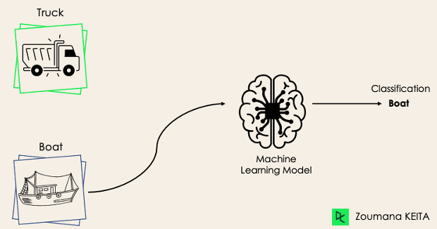
In a binary classification task, the goal is to classify the input data into two mutually exclusive categories. The training data in such a situation is labeled in a binary format: true and false; positive and negative; O and 1; spam and not spam, etc. depending on the problem being tackled. For instance, we might want to detect whether a given image is a truck or a boat. 

Logistic Regression and Support Vector Machines algorithms are natively designed for binary classifications. However, other algorithms such as K-Nearest Neighbors and Decision Trees can also be used for binary classification. 

Multi-Class Classification

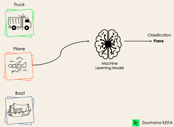
The multi-class classification, on the other hand, has at least two mutually exclusive class labels, where the goal is to predict to which class a given input example belongs to. In the following case, the model correctly classified the image to be a plane. 

Most of the binary classification algorithms can be also used for multi-class classification. These algorithms include but are not limited to:

• Random Forest
• Naive Bayes 
• K-Nearest Neighbors 
• Gradient Boosting 
• SVM
• Logistic Regression.

But wait! Didn’t you say that SVM and Logistic Regression do not support multi-class classification by default? 

→ That’s correct. However, we can apply binary transformation approaches such as one-versus-one and one-versus-all to adapt native binary classification algorithms for multi-class classification tasks.

One-versus-one: this strategy trains as many classifiers as there are pairs of labels. If we have a 3-class classification, we will have three pairs of labels, thus three classifiers, as shown below. 

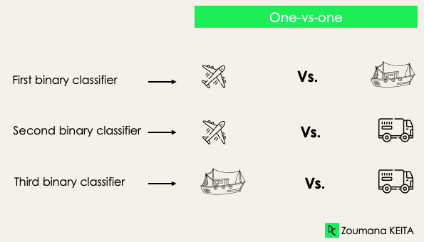
In general, for N labels, we will have Nx(N-1)/2 classifiers. Each classifier is trained on a single binary dataset, and the final class is predicted by a majority vote between all the classifiers. One-vs-one approach works best for SVM and other kernel-based algorithms. 

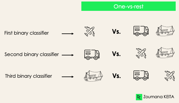
One-versus-rest: at this stage, we start by considering each label as an independent label and consider the rest combined as only one label. With 3-classes, we will have three classifiers. 

In general, for N labels, we will have N binary classifiers.

Multi-Label Classification

In multi-label classification tasks, we try to predict 0 or more classes for each input example. In this case, there is no mutual exclusion because the input example can have more than one label. 

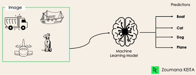
Such a scenario can be observed in different domains, such as auto-tagging in Natural Language Processing, where a given text can contain multiple topics. Similarly to computer vision, an image can contain multiple objects, as illustrated below: the model predicted that the image contains: a plane, a boat, a truck, and a dog.

It is not possible to use multi-class or binary classification models to perform multi-label classification. However, most algorithms used for those standard classification tasks have their specialized versions for multi-label classification. We can cite: 

• Multi-label Decision Trees
• Multi-label Gradient Boosting
• Multi-label Random Forests

Imbalanced Classification

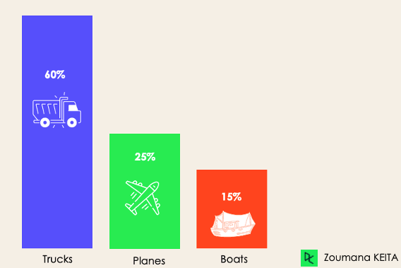
For the imbalanced classification, the number of examples is unevenly distributed in each class, meaning that we can have more of one class than the others in the training data. Let’s consider the following 3-class classification scenario where the training data contains: 60% of trucks, 25% of planes, and 15% of boats. 

The imbalanced classification problem could occur in the following scenario:

• Fraudulent transaction detections in financial industries
• Rare disease diagnosis 
• Customer churn analysis

Using conventional predictive models such as Decision Trees, Logistic Regression, etc. could not be effective when dealing with an imbalanced dataset, because they might be biased toward predicting the class with the highest number of observations, and considering those with fewer numbers as noise. 

So, does that mean that such problems are left behind?

Of course not! We can use multiple approaches to tackle the imbalance problem in a dataset. The most commonly used approaches include sampling techniques or harnessing the power of cost-sensitive algorithms. 

Sampling Techniques 

These techniques aim to balance the distribution of the original by: 

• Cluster-based Oversampling:
• Random undersampling: random elimination of examples from the majority class. 
• SMOTE Oversampling: random replication of examples from the minority class. 

Cost-Sensitive Algorithms 

These algorithms take into consideration the cost of misclassification. They aim to minimize the total cost generated by the models.

• Cost-sensitive Decision Trees.
• Cost-sensitive Logistic Regression. 
• Cost-sensitive Support Vector Machines.

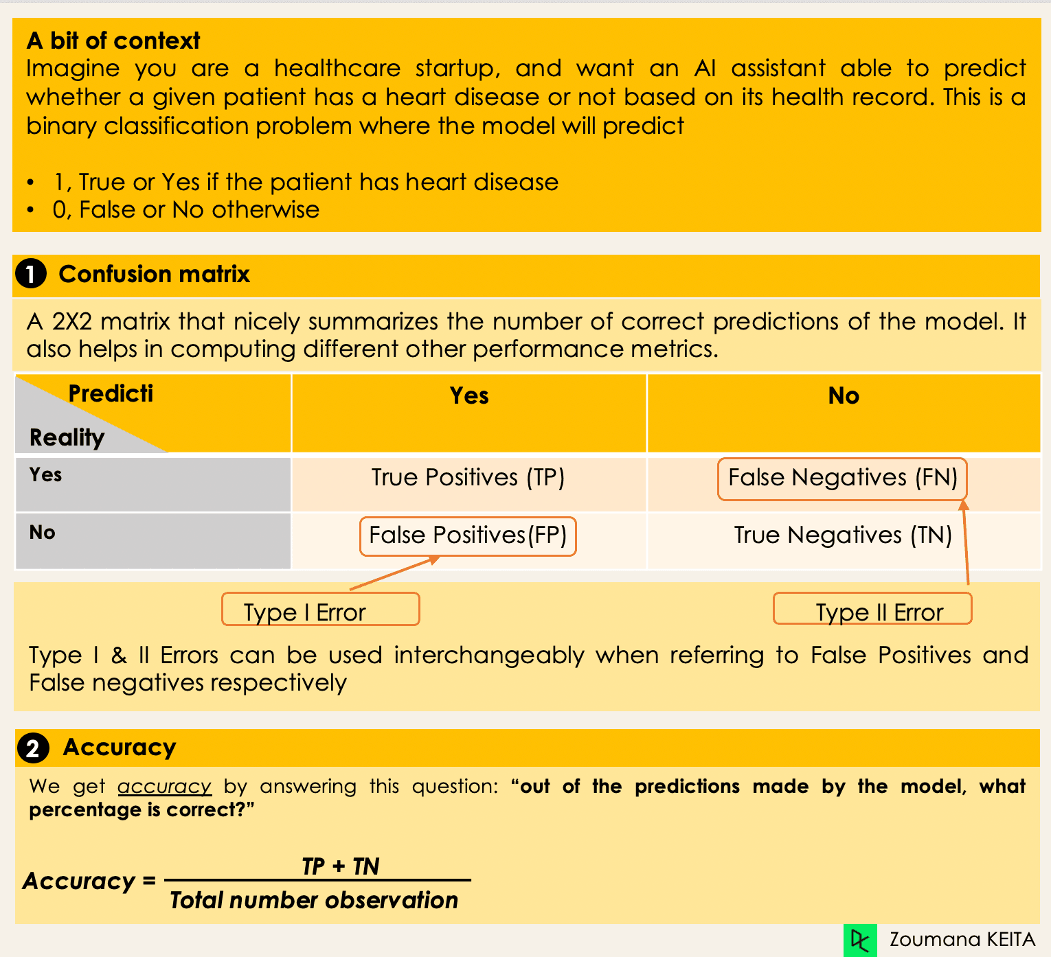
Metrics to Evaluate Machine Learning Classification Algorithms

Now that we have an idea of the different types of classification models, it is crucial to choose the right evaluation metrics for those models. In this section, we will cover the most commonly used metrics: accuracy, precision, recall, F1 score, and area under the ROC (Receiver Operating Characteristic) curve and AUC (Area Under the Curve). 

Deep Dive into Classification Algorithms  

We now have all the tools in hand to proceed with the implementation of some algorithms. This section will cover four algorithms and their implementation on the loans dataset to illustrate some of the previously covered concepts, especially for the imbalanced datasets using a binary classification task. We will focus on only four algorithms for simplicity’s sake. 

The goal is not to have the best possible model but to illustrate how to train each of the following algorithms. The source code is available on the DataCamp Workspace, where you can execute everything with one click.

Distribution of Loans in the Dataset 

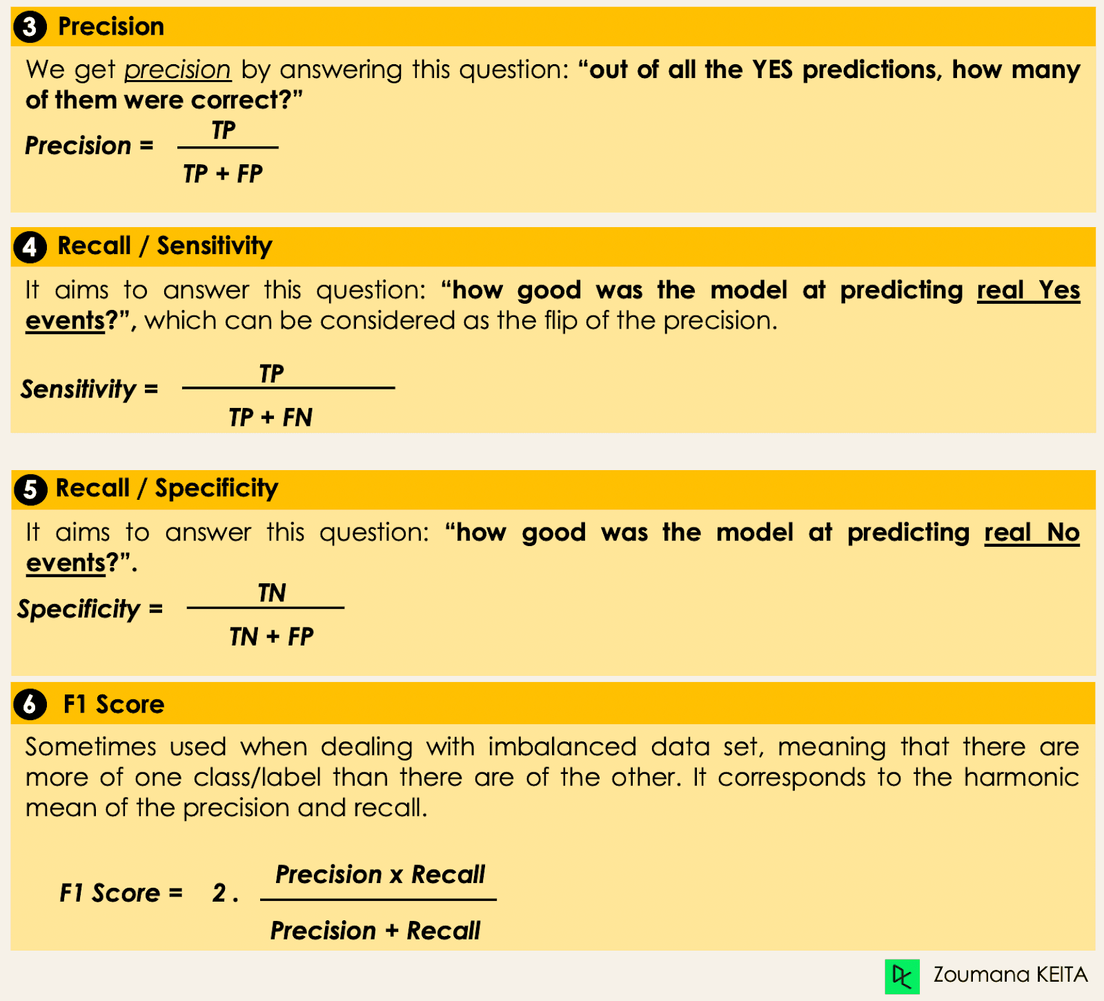
• Look at the first five observations in the dataset. 

import pandas as pd
loan_data = pd.read_csv("loan_data.csv")
loan_data.head()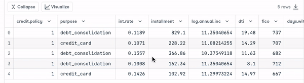

• Borrowers profile in the dataset. 

import matplotlib.pyplot as plt
# Helper function for data distribution
# Visualize the proportion of borrowers
def show_loan_distrib(data):
  count = ""
  if isinstance(data, pd.DataFrame):
      count = data["not.fully.paid"].value_counts()
  else:
      count = data.value_counts()


  count.plot(kind = 'pie', explode = [0, 0.1], 

              figsize = (6, 6), autopct = '%1.1f%%', shadow = True)
  plt.ylabel("Loan: Fully Paid Vs. Not Fully Paid")
  plt.legend(["Fully Paid", "Not Fully Paid"])
  plt.show()


# Visualize the proportion of borrowers
show_loan_distrib(loan_data)

From the graphic above, we notice that 84% of the borrowers paid their loans back, and only 16% didn’t pay them back, which makes the dataset really imbalanced.

Variable Types

Before further, we need to check the variables’ type so that we can encode those that need to be encoded. 

We notice that all the columns are continuous variables, except the purpose attribute, which needs to be encoded. 

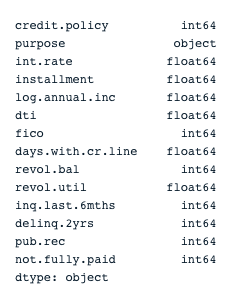
# Check column types
print(loan_data.dtypes)

encoded_loan_data = pd.get_dummies(loan_data, prefix="purpose",   

                                   drop_first=True)
print(encoded_loan_data.dtypes)

Separate data into train and test

X = encoded_loan_data.drop('not.fully.paid', axis = 1)
y = encoded_loan_data['not.fully.paid']


X_train, X_test, y_train, y_test = train_test_split(X, y, test_size=0.30, 

                                           stratify = y, random_state=2022)

Application of the Sampling Strategies 

We will explore two sampling strategies here: random undersampling, and SMOTE oversampling.

Random Undersampling 

We will undersample the majority class, which corresponds to the “fully paid” (class 0). 

X_train_cp = X_train.copy()
X_train_cp['not.fully.paid'] = y_train
y_0 = X_train_cp[X_train_cp['not.fully.paid'] == 0]
y_1 = X_train_cp[X_train_cp['not.fully.paid'] == 1]
y_0_undersample = y_0.sample(y_1.shape[0])
loan_data_undersample = pd.concat([y_0_undersample, y_1], axis = 0)


# Visualize the proportion of borrowers
show_loan_distrib(loan_data_undersample)

SMOTE Oversampling

Perform oversampling on the minority class

smote = SMOTE(sampling_strategy='minority')
X_train_SMOTE, y_train_SMOTE = smote.fit_resample(X_train,y_train)
# Visualize the proportion of borrowers
show_loan_distrib(y_train_SMOTE)

After applying the sampling strategies, we observe that the dataset is equally distributed across the different types of borrowers.

Application of Some Machine Learning Classification Algorithms

This section will apply these two classification algorithms to the SMOTE smote sampled dataset. The same training approach can be applied to undersampled data as well. 

Logistic Regression 

This is an explainable algorithm. It classifies a data point by modeling its probability of belonging to a given class using the sigmoid function. 

X = loan_data_undersample.drop('not.fully.paid', axis = 1)
y = loan_data_undersample['not.fully.paid']
X_train, X_test, y_train, y_test = train_test_split(X, y, test_size=0.15, stratify = y, random_state=2022)
logistic_classifier = LogisticRegression()
logistic_classifier.fit(X_train, y_train)
y_pred = logistic_classifier.predict(X_test)
print(confusion_matrix(y_test,y_pred))
print(classification_report(y_test,y_pred))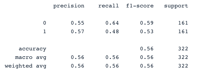

Support Vector Machines 

This algorithm can be used for both classification and regression. It learns to draw the hyperplane (decision boundary) by using the margin to maximization principle. This decision boundary is drawn through the two closest support vectors. 

SVM provides a transformation strategy called kernel tricks used to project non-learner separable data onto a higher dimension space to make them linearly separable. 

from sklearn.svm import SVC
svc_classifier = SVC(kernel='linear')
svc_classifier.fit(X_train, y_train)


# Make Prediction & print the result
y_pred = svc_classifier.predict(X_test)

print(classification_report(y_test,y_pred))

These results can be of course improved with more feature engineering and fine-tuning. But they are better than using the original imbalanced data. 

XGBoost

This algorithm is an extension of a well-known algorithm called gradient-boosted trees. It is a great candidate not only for combating overfitting but also for speed and performance.

To not make it longer, you can refer to Machine Learning with Tree-Based Models in Python and  Machine Learning with Tree-Based Models in R. From these courses, you will learn how to use both Python and R to implement tree-based models. 

Conclusion

This conceptual blog covered the main aspect of classifications in Machine learning and also provided you with some examples of different domains they are applied to. Finally, it covered the implementation of Logistic Regression and Support Vector Machine after performing the undersampling and SMOTE oversampling strategies to generate a balanced dataset for the models’ training. 

We hope it helped you have a better understanding of this topic of classification in Machine Learning. You can further your learning by following the Machine Learning Scientist with Python track,  which covers both supervised, unsupervised and deep learning. It also provides a good introduction to natural language processing, image processing, Spark, and Keras.