Introduction

Machine learning is a powerful tool for making predictions and finding patterns in data. However, building accurate models is not always straightforward. One of the main challenges in machine learning is finding the right balance between overfitting and underfitting.

Overfitting occurs when a model is too complex and fits too closely to the training data, resulting in poor performance on new data. Underfitting occurs when a model is too simple and fails to capture the underlying patterns in the data, also resulting in poor performance.

The Goldilocks Principle suggests that there is a “just right” level of complexity that achieves the best performance on new data.

In this article, we’ll explore the causes of overfitting and underfitting, and techniques for addressing them. We’ll also discuss the Goldilocks Principle and how it can be applied to machine learning. By finding the optimal balance between overfitting and underfitting, we can build models that generalize well to new data and make accurate predictions.

Overfitting

Overfitting occurs when a model becomes too complex and starts to memorize the training data instead of learning the underlying patterns. This can lead to the model performing well on the training data but poorly on new, unseen data.

A common example of overfitting is when a model fits the noise in the data instead of the underlying pattern. For instance, consider a dataset of housing prices where the target variable is the price of a house. One of the features in the dataset is the zip code of the house. If the model is too complex, it may start to memorize the housing prices of each zip code, including the noise in the data, instead of learning the underlying relationship between the zip code and the housing price.

Another example of overfitting is when a model is trained on a small dataset. In this case, the model may start to memorize the training data instead of learning the underlying patterns, leading to poor performance on new, unseen data.

To illustrate this, consider a model trained to classify images of cats and dogs. If the model is trained on a small dataset of only a few hundred images, it may start to memorize the training data instead of learning the underlying patterns that distinguish cats from dogs. This can lead to poor performance on new, unseen data, where the model may misclassify images of cats as dogs or vice versa.

In both of these examples, the model is too complex and is overfitting the training data, leading to poor performance on new, unseen data. In the next section, we will explore the various factors that can contribute to overfitting and techniques for addressing it.

Causes and Addressing Overfitting

Overfitting can occur due to various factors, such as the complexity of the model, the size of the dataset, and the noise in the data. Here are some techniques for addressing overfitting:

1. Regularization: Regularization is a technique that adds a penalty term to the loss function of the model to prevent it from overfitting. The penalty term adds a constraint on the weights of the model, making them smaller and reducing the complexity of the model. Two common types of regularization are L1 regularization and L2 regularization.
2. Early stopping: Early stopping is a technique where the training of the model is stopped when the performance on a validation set starts to degrade. This prevents the model from overfitting by finding the optimal point where the model has learned the underlying patterns but has not started to memorize the training data.
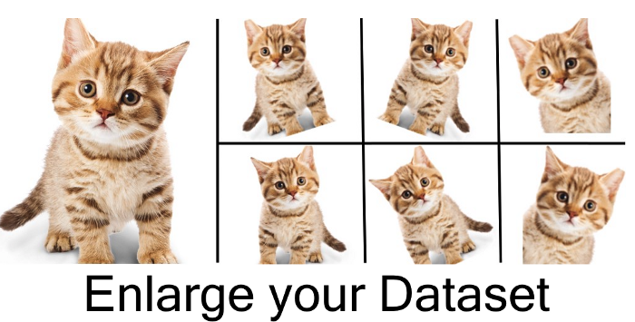
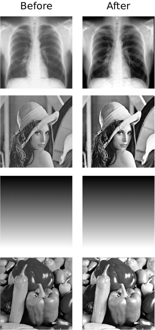
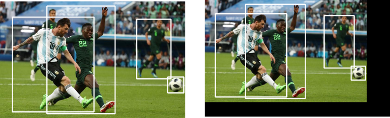
3. Data augmentation: Data augmentation is a technique where new training data is generated by applying various transformations to the existing data, such as flipping or rotating images. This increases the size of the dataset and helps the model learn the underlying patterns instead of memorizing the training data.
4. Dropout: Dropout is a technique where random nodes in the model are temporarily removed during training. This prevents the model from relying too much on any single node or feature, forcing it to learn more robust features that generalize well to new, unseen data.

In summary, overfitting can occur due to various factors, such as the complexity of the model and the size of the dataset. Regularization, early stopping, data augmentation, and dropout are some techniques for addressing overfitting and building machine learning models that can generalize well to new, unseen data.

Underfitting

Underfitting occurs when a model is too simple and is unable to capture the underlying patterns in the data. This can lead to poor performance on both the training data and new, unseen data.

A common example of underfitting is when a linear model is used to fit a non-linear relationship between the features and the target variable. In this case, the linear model may not be able to capture the non-linear relationship, leading to poor performance on both the training data and new, unseen data.

Another example of underfitting is when a model is not trained for long enough. In this case, the model may not have enough time to learn the underlying patterns in the data, leading to poor performance on both the training data and new, unseen data.

To illustrate this, consider a model trained to predict the price of a house based on the number of bedrooms and bathrooms. If the model is too simple, it may only consider the number of bedrooms and bathrooms and ignore other important features, such as the location of the house and the size of the lot. This can lead to poor performance on both the training data and new, unseen data.

In summary, underfitting occurs when a model is too simple and is unable to capture the underlying patterns in the data. This can lead to poor performance on both the training data and new, unseen data. In the next section, we will explore the various factors that can contribute to underfitting and techniques for addressing it.

Causes and Addressing Underfitting

Underfitting can occur due to various factors, such as the simplicity of the model, the lack of relevant features, and insufficient training. Here are some techniques for addressing underfitting:

1. Increasing model complexity: If a model is too simple and is unable to capture the underlying patterns in the data, one approach is to increase the complexity of the model. This can be done by adding more layers or nodes to a neural network, increasing the polynomial degree of a regression model, or using a more complex algorithm.
2. Adding relevant features: If a model is unable to capture the underlying patterns in the data due to a lack of relevant features, one approach is to add additional features to the dataset. This can be done by collecting more data or engineering new features from existing data.
3. Increasing training time: If a model is unable to capture the underlying patterns in the data due to insufficient training, one approach is to increase the training time. This can be done by training the model for longer or using more training data.
4. Ensemble methods: Ensemble methods are a technique where multiple models are trained on the same dataset and their predictions are combined to make a final prediction. This can help address underfitting by combining the strengths of multiple models to capture the underlying patterns in the data.

In summary, underfitting can occur due to various factors, such as the simplicity of the model, the lack of relevant features, and insufficient training. Increasing model complexity, adding relevant features, increasing training time, and ensemble methods are some techniques for addressing underfitting and building machine learning models that can capture the underlying patterns in the data.

Balancing Overfitting and Underfitting

The goal of building a machine learning model is to find the right balance between overfitting and underfitting. This balance is known as the bias-variance tradeoff.

Bias refers to the error that is introduced by approximating a real-world problem with a simpler model. High bias models are typically simple models that underfit the data.

Variance refers to the error that is introduced by the model’s sensitivity to small fluctuations in the training data. High variance models are typically complex models that overfit the data.

A good model should have low bias and low variance. This means that the model should capture the underlying patterns in the data without being overly sensitive to noise or small fluctuations in the data.

To find the right balance between overfitting and underfitting, it is important to tune the model’s hyperparameters. Hyperparameters are parameters that are not learned during training, but are set by the user before training. Examples of hyperparameters include the learning rate, the number of hidden layers in a neural network, and the regularization strength.

One common approach to balancing overfitting and underfitting is to use a validation set. A validation set is a portion of the training data that is set aside for testing the model during training. By evaluating the model’s performance on the validation set, the user can adjust the hyperparameters to find the right balance between overfitting and underfitting.

Another approach to balancing overfitting and underfitting is to use regularization. Regularization is a technique that penalizes large weights in the model, which can help prevent overfitting. Common forms of regularization include L1 and L2 regularization, which add a penalty term to the loss function to encourage the model to have smaller weights.

In summary, balancing overfitting and underfitting is a critical part of building machine learning models that can capture the underlying patterns in the data. Tuning the model’s hyperparameters, using a validation set, and regularization are some techniques for finding the right balance between overfitting and underfitting.

Conclusion

In this article, we explored the concepts of overfitting and underfitting in machine learning. Overfitting occurs when a model is overly complex and captures noise in the training data, while underfitting occurs when a model is too simple and fails to capture the underlying patterns in the data.

We discussed the causes of overfitting and underfitting and presented several techniques for addressing these issues, including regularization, early stopping, and increasing the complexity of the model.

Finding the right balance between overfitting and underfitting is a critical part of building machine learning models that can generalize to new data. Tuning the model’s hyperparameters and using a validation set can help find this balance.

Ultimately, the success of a machine learning model depends on its ability to accurately predict on new data. By understanding the concepts of overfitting and underfitting, and how to address them, we can build models that are more accurate and effective in solving real-world problems.

What is Image Classification?

Classification between objects is a fairly easy task for us, but it has proved to be a complex one for machines and therefore image classification has been an important task within the field of computer vision.
Image classification refers to the labeling of images into one of a number of predefined classes.
There are potentially n number of classes in which a given image can be classified. Manually checking and classifying images could be a tedious task especially when they are massive in number (say 10,000) and therefore it will be very useful if we could automate this entire process using computer vision.

Some examples of image classification include:

• Labeling an x-ray as cancer or not (binary classification).
• Classifying a handwritten digit (multiclass classification).
• Assigning a name to a photograph of a face (multiclass classification).

The advancements in the field of autonomous driving also serve as a great example of the use of image classification in the real-world. For example, we can build an image classification model that recognizes various objects, such as other vehicles, pedestrians, traffic lights, and signposts on the road.

Now that we have a fair idea of what image classification comprises of, let’s start analyzing the image classification pipeline.

Structure of an Image Classification Task

1. Image Preprocessing – The aim of this process is to improve the image data(features) by suppressing unwanted distortions and enhancement of some important image features so that our Computer Vision models can benefit from this improved data to work on.
2. Detection of an object – Detection refers to the localization of an object which means the segmentation of the image and identifying the position of the object of interest.
3. Feature extraction and Training– This is a crucial step wherein statistical or deep learning methods are used to identify the most interesting patterns of the image, features that might be unique to a particular class and that will, later on, help the model to differentiate between different classes. This process where the model learns the features from the dataset is called model training.
4. Classification of the object – This step categorizes detected objects into predefined classes by using a suitable classification technique that compares the image patterns with the target patterns.

Let’s discuss the most crucial step which is image preprocessing, in detail!

Image Pre-processing

Pre-processing is a common name for operations with images at the lowest level of abstraction — both input and output are intensity images.

Need for Image-Preprocessing
Computers are able to perform computations on numbers and is unable to interpret images in the way that we do. We have to somehow convert the images to numbers for the computer to understand.
The aim of pre-processing is an improvement of the image data that suppresses unwilling distortions or enhances some image features important for further processing.

How computers see an ‘8’
Image Source: Link

Steps for image pre-processing:

• Read image
• Resize image
• Data Augmentation
  • Gray scaling of image
  • Reflection
  • Gaussian Blurring
  • Histogram Equalization
  • Rotation
  • Translation

Step 1
Reading Image
In this step, we simply store the path to our image dataset into a variable and then we create a function to load folders containing images into arrays so that computers can deal with it.

Sample code for reading an image dataset with 2 classes:

# importing libraries
from pathlib import Path
import glob
import pandas as pd

# reading images from path
images_dir = Path('img')
images = images_dir.glob("*.tif")

train_data = []

counter = 0
for img in images:
  counter += 1
  if counter <= 130:
    train_data.append((img,1))
  else:
    train_data.append((img,0))
 
# converting data into pandas dataframe for easy visualization 
train_data = pd.DataFrame(train_data,columns=['image','label'],index = None)
PythonCopy

Step 2.
Resize image
Some images captured by a camera and fed to our AI algorithm vary in size, therefore, we should establish a base size for all images fed into our AI algorithms by resizing them.

Sample code for resizing images into 229×229 dimensions:

img = cv2.resize(img, (229,229))
PythonCopy

Step 3
Data Augmentation
Data augmentation is a way of creating new ‘data’ with different orientations. The benefits of this are two-fold, the first being the ability to generate ‘more data’ from limited data and secondly, it prevents overfitting.

Image Source and Credit: Link

Data Augmentation Techniques:

1. Gray Scaling
   The image will be converted to gray scale (range of gray shades from white to black) the computer will assign each pixel a value based on how dark it is. All the numbers are put into an array and the computer does computations on that array.

Sample code to convert an RGB(3 channels) image into a Gray scale image:

import cv2
img = cv2.cvtColor(img, cv2.COLOR_BGR2GRAY)
PythonCopy

RGB Image

Grayscale Image:

Images Source: Link

2. Reflection/Flip
   You can flip images horizontally and vertically. Some frameworks do not provide function for vertical flips. But, a vertical flip is equivalent to rotating an image by 180 degrees and then performing a horizontal flip.

Sample Code:

# horizontal flip
img = cv2.flip(img, 0) 

# vertical flip
img = cv2.flip(img,1)
PythonCopy

Image showing horizontal reflection
Image Source: Link

3. Gaussian Blurring
   Gaussian blur (also known as Gaussian smoothing) is the result of blurring an image by a Gaussian function. It is a widely used effect in graphics software, typically to reduce image noise.

Sample Code:

from scipy import ndimage
img = ndimage.gaussian_filter(img, sigma= 5.11)
PythonCopy

Image with blur radius = 5.1
Image Source:Link

4. Histogram Equalization
   Histogram equalization is another image processing technique to increase global contrast of an image using the image intensity histogram. This method needs no parameter, but it sometimes results in an unnatural looking image.

Sample Code

# histogram equalization function
def hist(img):
  img_to_yuv = cv2.cvtColor(img,cv2.COLOR_BGR2YUV)
  img_to_yuv[:,:,0] = cv2.equalizeHist(img_to_yuv[:,:,0])
  hist_equalization_result = cv2.cvtColor(img_to_yuv, cv2.COLOR_YUV2BGR)
  return hist_equalization_result
PythonCopy

Image Credit and Source: Link

5. Rotation
   This is yet another image augmentation technique. Rotating an image might not preserve its original dimensions (depending on what angle you choose to rotate it with )

Sample Code

import random
# function for rotation
def rotation(img):
  rows,cols = img.shape[0],img.shape[1]
  randDeg = random.randint(-180, 180)
  matrix = cv2.getRotationMatrix2D((cols/2, rows/2), randDeg, 0.70)
  rotated = cv2.warpAffine(img, matrix, (rows, cols), borderMode=cv2.BORDER_CONSTANT,borderValue=(144, 159, 162))
  return rotated     
PythonCopy

The images are rotated by 90 degrees clockwise with respect to the previous one, as we move from left to right.
Image Source and Credit: Link

6. Translation
   Translation just involves moving the image along the X or Y direction (or both).
   This method of augmentation is very useful as most objects can be located at almost anywhere in the image. This forces our feature extractor to look everywhere.

Sample Code

img = cv2.warpAffine(img, np.float32([[1, 0, 84], [0, 1, 56]]), (img.shape[0], img.shape[1]),
borderMode=cv2.BORDER_CONSTANT,borderValue=(144, 159, 162))
PythonCopy

Image Source and Credit:Link

Image Classification Techniques

We will start with some statistical machine learning classifiers like Support Vector Machine and Decision Tree and then move on to deep learning architectures like Convolutional Neural Networks.

To support their performance analysis, the results from an Image classification task used to differentiate lymphoblastic leukemia cells from non-lymphoblastic ones have been provided. The features have been extracted using a convolutional neural network, which will also be discussed as one of our classifiers. This is because deep learning models have achieved state of the art results in the feature extraction process.

Different classifiers are then added on top of this feature extractor to classify images.

1. Support Vector Machines

It is a supervised machine learning algorithm used for both regression and classification problems.
When used for classification purposes, it separates the classes using a linear boundary.

Image Source: Link

It builds a hyper-plane or a set of hyper-planes in a high dimensional space and good separation between the two classes is achieved by the hyperplane that has the largest distance to the nearest training data point of any class.
The real power of this algorithm depends on the kernel function being used.
The most commonly used kernels are:

• Linear Kernel
• Gaussian Kernel
• Polynomial Kernel

Code Snippet:

This is the base model/feature extractor using Convolutional Neural Network, using Keras with Tensorflow backend

model = Sequential()
model.add(Conv2D(16,(5,5),padding='valid',input_shape = X_train.shape[1:]))
model.add(Activation('relu'))
model.add(MaxPooling2D(pool_size=(2,2),strides=2,padding = 'valid'))
model.add(Dropout(0.4))
model.add(Conv2D(32,(5,5),padding='valid'))
model.add(Activation('relu'))
model.add(MaxPooling2D(pool_size=(2,2),strides=2,padding = 'valid'))
model.add(Dropout(0.6))
model.add(Conv2D(64,(5,5),padding='valid'))
model.add(Activation('relu'))
model.add(Dropout(0.8))
model.add(Flatten())
model.add(Dense(2))
model.add(Activation('softmax'))

model_feat = Model(inputs=model.input,outputs=model.get_layer('dense_1').output)
feat_train = model_feat.predict(X_train)
PythonCopy

Fitting of SVM as a classifier

svm = SVC(kernel='rbf')
svm.fit(feat_train,np.argmax(y_train,axis=1))

svm.score(feat_test,np.argmax(y_test,axis=1))
PythonCopy

Accuracy score on test data: 85.68

Link to know more about SVM

2. Decision Trees

It is also a supervised machine learning algorithm, which at its core is the tree data structure only, using a couple of if/else statements on the features selected.
Decision trees are based on a hierarchical rule-based method and permits the acceptance and rejection of class labels at each intermediary stage/level.

Image Source: Link

This method consists of 3 parts:

• Partitioning the nodes
• Finding the terminal nodes
• Allocation of the class label to terminal node

Code
Feature Extractor

model = Sequential()
model.add(Conv2D(16,(5,5),padding='valid',input_shape = X_train.shape[1:]))
model.add(Activation('relu'))
model.add(MaxPooling2D(pool_size=(2,2),strides=2,padding = 'valid'))
model.add(Dropout(0.4))
model.add(Conv2D(32,(5,5),padding='valid'))
model.add(Activation('relu'))
model.add(MaxPooling2D(pool_size=(2,2),strides=2,padding = 'valid'))
model.add(Dropout(0.6))
model.add(Conv2D(64,(5,5),padding='valid'))
model.add(Activation('relu'))
model.add(Dropout(0.8))
model.add(Flatten())
model.add(Dense(2))
model.add(Activation('softmax'))

model_feat = Model(inputs=model.input,outputs=model.get_layer('dense_2').output)
feat_train = model_feat.predict(X_train)
PythonCopy

Decision Tree Classifier

dt = DecisionTreeClassifier(criterion = "entropy", random_state = 100,max_depth=3, min_samples_leaf=5)
dt.fit(feat_train,np.argmax(y_train,axis=1))

dt.score(feat_test,np.argmax(y_test,axis=1))
PythonCopy

Accuracy on test set: 84.61

Link to know more about Decision Trees

3. K Nearest Neighbor

The k-nearest neighbor is by far the most simple machine learning algorithm.
This algorithm simply relies on the distance between feature vectors and classifies unknown data points by finding the most common class among the k-closest examples.

Image Source: Link

Here we can see there are two categories of images and that each of the data points within each respective category are grouped relatively close together in an n-dimensional space.

In order to apply the k-nearest Neighbor classification, we need to define a distance metric or similarity function. Common choices include the Euclidean distance and Manhattan distance

Code
Base Model/feature extractor

model = Sequential()
model.add(Conv2D(16,(5,5),padding='valid',input_shape = X_train.shape[1:]))
model.add(Activation('relu'))
model.add(MaxPooling2D(pool_size=(2,2),strides=2,padding = 'valid'))
model.add(Dropout(0.4))
model.add(Conv2D(32,(5,5),padding='valid'))
model.add(Activation('relu'))
model.add(MaxPooling2D(pool_size=(2,2),strides=2,padding = 'valid'))
model.add(Dropout(0.6))
model.add(Conv2D(64,(5,5),padding='valid'))
model.add(Activation('relu'))
model.add(Dropout(0.8))
model.add(Flatten())
model.add(Dense(2))
model.add(Activation('softmax'))

model_feat = Model(inputs=model.input,outputs=model.get_layer('dense_2').output)
feat_train = model_feat.predict(X_train)
PythonCopy

KNN classifier

knn = KNeighborsClassifier(n_neighbors=12)
knn.fit(feat_train,np.argmax(y_train,axis=-1))

knn.score(feat_test,np.argmax(y_test,axis=1))
PythonCopy

Accuracy on test set: 86.32

Link to explore KNN

4. Artificial Neural Networks

Inspired by the properties of biological neural networks, Artificial Neural Networks are statistical learning algorithms and are used for a variety of tasks, from relatively simple classification tasks to computer vision and speech recognition.
ANNs are implemented as a system of interconnected processing elements, called nodes, which are functionally analogous to biological neurons.The connections between different nodes have numerical values, called weights, and by altering these values in a systematic way, the network is eventually able to approximate the desired function.

Images Credit and Source: Link

The hidden layers can be thought of as individual feature detectors, recognizing more and more complex patterns in the data as it is propagated throughout the network. For example, if the network is given a task to recognize a face, the first hidden layer might act as a line detector, the second hidden takes these lines as input and puts them together to form a nose, the third hidden layer takes the nose and matches it with an eye and so on, until finally the whole face is constructed. This hierarchy enables the network to eventually recognize very complex objects.

Code
ANN as feature extractor using softmax classifier

model_ann = Sequential()
model_ann.add(Dense(16, input_shape=X_train.shape[1:], activation='relu'))
model_ann.add(Dropout(0.4))
model_ann.add(Dense(32, activation='relu'))
model_ann.add(Dropout(0.6))
model_ann.add(Flatten())
model_ann.add(Dense(2, activation='softmax'))

model_ann.compile(loss='binary_crossentropy', optimizer='adam', metrics=['accuracy'])

history = model_ann.fit(X_train, y_train,epochs=100,batch_size=100)
history
PythonCopy

Accuracy on test data: 83.1
This result has been recorded for 100 epochs, and the accuracy improves as the epochs are further increased.

Link to study ANN in detail

5. Convolutional Neural Networks

Convolutional neural networks (CNN) is a special architecture of artificial neural networks. CNNs uses some of its features of visual cortex and have therefore achieved state of the art results in computer vision tasks.

Let’s cover the use of CNN in more detail.

Convolutional neural networks are comprised of two very simple elements, namely convolutional layers and pooling layers.
Although simple, there are near-infinite ways to arrange these layers for a given computer vision problem.
The elements of a convolutional neural network, such as convolutional and pooling layers, are relatively straightforward to understand.
The challenging part of using convolutional neural networks in practice is how to design model architectures that best use these simple elements.

Image Source: Link

Code
CNN as feature extractor using softmax classifier

model = Sequential()
model.add(Conv2D(16,(5,5),padding='valid',input_shape = X_train.shape[1:]))
model.add(Activation('relu'))
model.add(MaxPooling2D(pool_size=(2,2),strides=2,padding = 'valid'))
model.add(Dropout(0.4))
model.add(Conv2D(32,(5,5),padding='valid'))
model.add(Activation('relu'))
model.add(MaxPooling2D(pool_size=(2,2),strides=2,padding = 'valid'))
model.add(Dropout(0.6))
model.add(Conv2D(64,(5,5),padding='valid'))
model.add(Activation('relu'))
model.add(Dropout(0.8))
model.add(Flatten())
model.add(Dense(2))
model.add(Activation('softmax'))

batch_size = 100
epochs= 100

optimizer = keras.optimizers.rmsprop(lr = 0.0001, decay = 1e-6)

model.compile(loss = 'binary_crossentropy',optimizer = optimizer, metrics = ['accuracy',keras_metrics.precision(), keras_metrics.recall()])

history = model.fit(X_train,y_train,steps_per_epoch = int(len(X_train)/batch_size),epochs=epochs)
history
PythonCopy

Accuracy on test data with 100 epochs: 87.11
Since this model gave the best result amongst all, it was trained longer and it achieved 91% accuracy with 300 epochs.

Link for more on CNN

Performance evaluation

CLASSIFIER	ACCURACY	PRECISION	RECALL	ROC
SVM	85.68%	0.86	0.87	0.86
Decision Trees	84.61%	0.85	0.84	0.82
KNN	86.32%	0.86	0.86	0.88
ANN(for 100 epochs)	83.10%	0.88	0.87	0.88
CNN(for 300 epochs)	91.11%	0.93	0.89	0.97

Conclusion

We can conclude from the performance table, that Convolutional Neural networks deliver the best results in computer vision tasks.

If you liked the content of this post, do share it with others!