
Simply put, Machine Learning (ML) is the process of employing algorithms to help computer systems progressively improve their performance for some specific task. Software-based ML can be traced back to the 1950’s, but the number and ubiquity of ML algorithms has exploded since the early 2000’s, mainly due to the rising popularity of the Python programming language, which continues to drive advances in ML.
The reigning ML algorithm champ is arguably Python’s scikit-learn package, which offers simple and easy syntax paired with a treasure trove of multiple algorithms. While some algorithms are more appropriate for specific tasks, others are widely applicable to any project.
In this article, I’ll show you the top 10 machine learning algorithms that always save my day!
Before You Start: Install The Top 10 Algorithms Python Environment
To follow along with the code in this article, you can download and install our pre-built Top 10 Algorithms environment, which contains a version of Python 3.9 and the packages used in this post.
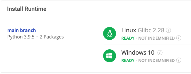
In order to download this ready-to-use Python environment, you will need to create an ActiveState Platform account. Just use your GitHub credentials or your email address to register. Signing up is easy and it unlocks the ActiveState Platform’s many benefits for you!
Or you could also use our State tool to install this runtime environment.
For Windows users, run the following at a CMD prompt to automatically download and install our CLI, the State Tool along with the Top 10 Algorithms into a virtual environment:
powershell -Command "& $([scriptblock]::Create((New-Object Net.WebClient).DownloadString('https://platform.activestate.com/dl/cli/install.ps1'))) -activate-default Pizza-Team/Top-Algorithms"
For Linux users, run the following to automatically download and install our CLI, the State Tool along with the Top 10 Algorithms into a virtual environment:
sh <(curl -q https://platform.activestate.com/dl/cli/install.sh) --activate-default Pizza-Team/Top-Algorithms
Choosing A Dataset
To show how different algorithms work, we’ll apply them to a standard dataset. It has often been said that the results of an ML experiment are more dependent on the dataset you use than the algorithm you chose. With this in mind, we’ll choose a reputable classification dataset from Kaggle called “Titanic – Machine Learning from Disaster.”
Exploring a Dataset
By consulting the data dictionary on Kaggle, we can see that the dataset contains the following information:
| Variable | Definition | Key |
| survival | survival | 0 = No, 1 = Yes |
| pclass | ticket class | 1 = 1st, 2 = 2nd, 3 = 3rd |
| sex | sex | |
| age | age (in years) | |
| sibsp | # of siblings/spouses aboard the Titanic | |
| parch | # of parents/children aboard the Titanic | |
| ticket | ticket number | |
| fare | passenger fare | |
| cabin | cabin number | |
| embarked | port of embarkation | C = Cherbourg Q = Queenstown S = Southampton |
At this phase, you would typically perform an Exploratory Data Analysis on the dataset. If you’d like to deep-dive into this, you can pause this article and read my “Exploratory Data Analysis Using Python” blog and come right back.
Cleaning & Preparing a Dataset
Before we apply any algorithms against this data, it needs to be cleaned. This means weeding out missing values, transforming label data, normalizing values, and sometimes even dumping columns that we don’t need.
In the interest of time (and length), I’m going to gloss over this portion. If you want to read a more detailed approach to this, you can explore another one of my blogs: “How To Clean Machine Learning Datasets Using Pandas” from where I’ve taken some of the concepts used in this article.
Step 1: Drop Unnecessary Columns
Several columns either have missing data or too much textual information that we can’t easily use. We can drop them like this:
def drop_useless_columns(self):

   self.df.drop(['PassengerId'], axis=1, inplace=True)

   self.df.drop(['Name'], axis=1, inplace=True)

   self.df.drop(['Ticket'], axis=1, inplace=True)

   self.df.drop(['Cabin'], axis=1, inplace=True)
It is important to note that many of these columns could be put to use to further strengthen the result. However, that would involve a lot of pre-processing.
Step 2: Encode Labels
This step converts labels into comparable numeric data:
def one_hot_encode_columns(self):

   # Encode Pclass

   dummies = pd.get_dummies(self.df['Pclass'], prefix='route')

   self.df = pd.concat([self.df, dummies], axis=1)

   self.df.drop(['Pclass'], axis=1, inplace=True)


   # Encode Sex

   dummies = pd.get_dummies(self.df['Sex'], prefix='route')

   self.df = pd.concat([self.df, dummies], axis=1)

   self.df.drop(['Sex'], axis=1, inplace=True)


   # Encode Embarked

   dummies = pd.get_dummies(self.df['Embarked'], prefix='route')

   self.df = pd.concat([self.df, dummies], axis=1)

   self.df.drop(['Embarked'], axis=1, inplace=True)
Step 3: Fill in Missing Values
You can use self.df.isna().any() to find out if the dataset has missing or NaN columns:
Survived        False

Age              True

SibSp           False

Parch           False

Fare            False

route_1         False

route_2         False

route_3         False

route_female    False

route_male      False

route_C         False

route_Q         False

route_S         False

dtype: bool
As you can see, the age variable has missing values. We can fill those in by getting the average age of the entire dataset:
ef fill_in_nan(self):

   mean_age = self.df['Age'].mean()

   self.df['Age'].fillna(value=mean_age, inplace=True)
Step 4 – Splitting The Dataset
Now, let’s split the dataset into training and testing data using sklearn’s train_test_split:
@staticmethod

 def clean_and_split():

   base = Base()


   # clean

   base.drop_useless_columns()

   base.one_hot_encode_columns()

   base.fill_in_nan()


   # split

   return base.split()
Perfect! Now that we’ve cleaned up the data and split it, it’s time to learn – or rather, for the machine to learn!
Top ML Algorithms in Scikit-Learn
Decision Tree Algorithm
The Decision Tree algorithm is widely applicable to most scenarios, and can be surprisingly effective for such a simple algorithm. It requires minimal data preparation, and can even work with blank values. This algorithm focuses on learning simple decision rules inferred from the data. It then compiles them into a set of “if-then-else” decision rules:
from sklearn.tree import DecisionTreeClassifier

from base import Base


Xtrain, Xtest, ytrain, ytest = Base.clean_and_split()


model = DecisionTreeClassifier()

model.fit(Xtrain, ytrain)

ypred = model.predict(Xtest)


print("\n\nDecision Tree Accuracy Score:", Base.accuracy_score(ytest, ypred), "%")
And here’s the result:
[Running] python -u "/top-10-machine-learning-algorithms-sklearn/decision_tree.py"


Decision Tree Accuracy Score: 75.0 %


[Done] exited with code=0 in 1.248 seconds
Now, let’s chart a visualization of the tree itself. It’s quite easy to do since sklearn provides export_graphviz as part of its tree module:
from sklearn.tree import export_graphviz

dot_file = 'visualizations/decision_tree.dot'

export_graphviz(model, out_file=dot_file, feature_names=Xtrain.columns.values)
Now that you have the file, just convert it into a PNG image:
dot -Tpng decision_tree.dot -o decision_tree.png
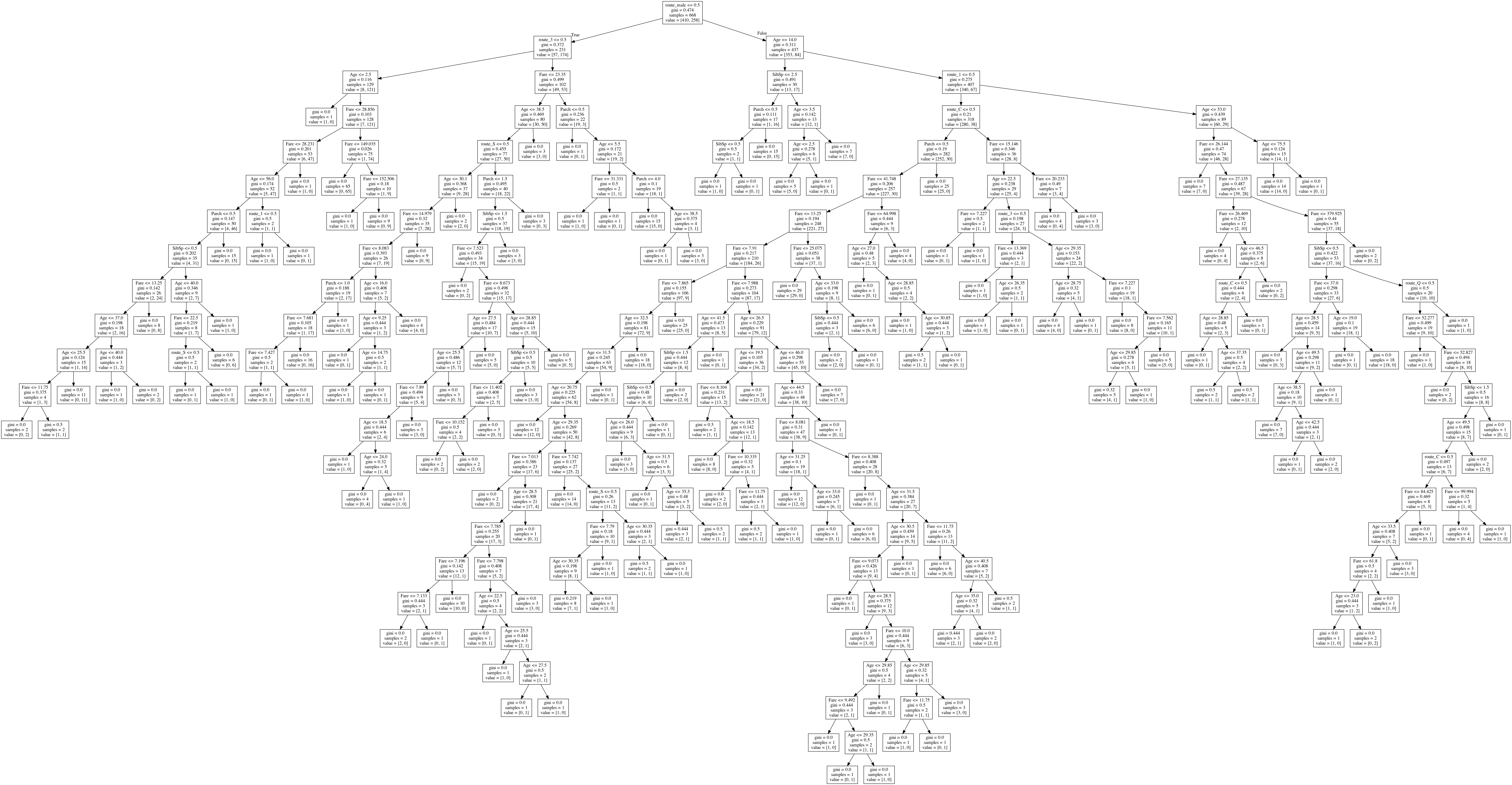
You can also view a more detailed version here.
Random Forest Classifier Algorithm
If you think one decision tree is great, imagine what a forest of them could do! That’s essentially what a Random Forest Classifier does. The classification starts off by using multiple trees with slightly different training data. The predictions from all of the trees are then averaged out, resulting in better performance than any single tree in the model.
Random Forests can be used to solve classification or regression problems. Let’s have a look at how it solves the following classification problem:
from sklearn.ensemble import RandomForestClassifier

from base import Base


Xtrain, Xtest, ytrain, ytest = Base.clean_and_split()


model = RandomForestClassifier()

model.fit(Xtrain, ytrain)

ypred = model.predict(Xtest)


print("\n\nRandom Forest Classifier Accuracy Score:", Base.accuracy_score(ytest, ypred), "%")
And now for the result:
[Running] python -u "/top-10-machine-learning-algorithms-sklearn/random_forest.py"

Random Forest Classifier Accuracy Score: 81.0 %

[Done] exited with code=0 in 1.106 seconds
K-Nearest Neighbor Algorithm
The k-nearest neighbor (KNN) algorithm is a simple and efficient algorithm that can be used to solve both classification and regression problems. If you know the saying, “birds of a feather flock together” you have the essence of KNN in a nutshell. It assumes that similar “things” exist in close proximity to each other.
Although you need to perform a certain amount of data cleansing before applying the algorithm, the benefits outweigh the burdens. Let’s have a look:
from sklearn.neighbors import KNeighborsClassifier

from base import Base


Xtrain, Xtest, ytrain, ytest = Base.clean_and_split()


model = KNeighborsClassifier(n_neighbors=7)

model.fit(Xtrain, ytrain)

ypred = model.predict(Xtest)


print("\n\nK-Nearest Neighbor Accuracy Score:", Base.accuracy_score(ytest, ypred), "%")
As you can see, you can tune the hyperparameters to achieve the highest accuracy. When the above code is executed with just 1 neighbor, the accuracy rate falls to 70%.
[Running] python -u "/top-10-machine-learning-algorithms-sklearn/knn.py"

K-Nearest Neighbor Accuracy Score: 74.0 %

[Done] exited with code=0 in 0.775 seconds
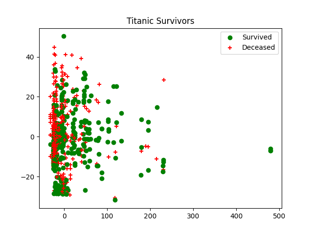
Now let’s visualize it. This part is a little tricky since we will need to reduce the model’s dimensions to be able to visualize the result on a scatter plot. You may want to read more about Principal Component Analysis (PCA), but for the purposes of this article, all you need to know is that PCA is used to reduce dimensionality while preserving the meaning of the data.
# Transforming n-features into 2

pca = PCA(n_components=2).fit(X)

pca_2d = pca.transform(X)


for i in range(0, pca_2d.shape[0]):

   if y[i] == 1:

       c1 = pl.scatter(pca_2d[i,0], pca_2d[i,1], c='g', marker='o')

   elif y[i] == 0:

       c2 = pl.scatter(pca_2d[i,0], pca_2d[i,1], c='r', marker='+')


pl.legend([c1, c2], ['Survived', 'Deceased'])

pl.title('Titanic Survivors')

plt.savefig('visualizations/knn.png')
Now let’s plot our data. We’ll use green dots for passengers who survived and red ones for passengers who did not:
Bagging Classifier Algorithm
Before we look into Bagging Classifiers, we must understand ensemble learning. In the previous example of Random Forests and Decision Trees, we learned that the former is an averaging of the results of the latter.
This is essentially what bagging is: it’s a paradigm in which multiple “weak” learners are trained in parallel to solve the same problem, and then combined to get better results.
from sklearn.svm import SVC

from sklearn.ensemble import BaggingClassifier

from base import Base


Xtrain, Xtest, ytrain, ytest = Base.clean_and_split()


model = BaggingClassifier(

 base_estimator=SVC(),

 n_estimators=10,

 random_state=0

)

model.fit(Xtrain, ytrain)

ypred = model.predict(Xtest)


print("\n\nBagging Accuracy Score:", Base.accuracy_score(ytest, ypred), "%")
In order to split up the data for multiple learners, we use a Linear Support Vector Classifier (SVC) to fit and divide the data as equally as possible. This means that no one set of data will lean on a column too much or have too much variability between the data.
Let’s see what happens:
[Running] python -u "/top-10-machine-learning-algorithms-sklearn/bagging.py"

Bagging Accuracy Score: 72.0 %

[Done] exited with code=0 in 1.302 seconds
Boosting Classifier Algorithm
Boosting is very similar to bagging in the sense that it averages out the results of multiple weak learners. However, in the case of boosting, these learners are executed in a sequential manner such that the latest model depends on the previous one. This leads to lower bias, meaning that it can handle a larger variance of data.
from xgboost.sklearn import XGBClassifier

from base import Base


Xtrain, Xtest, ytrain, ytest = Base.clean_and_split()


model = XGBClassifier()

model.fit(Xtrain, ytrain)

ypred = model.predict(Xtest)


print("\n\nXG Boost Classifier Accuracy Score:", Base.accuracy_score(ytest, ypred), "%")
And here is the result:
[Running] python -u "/top-10-machine-learning-algorithms-sklearn/xgboost.py"

Bagging Accuracy Score: 77.0 %

[Done] exited with code=0 in 1.302 seconds
Naive Bayes Algorithm
It’s time to remember your high school course in probability. The Naive Bayes algorithm determines the probability of each feature set and uses that to determine the probability of the classification itself.
Here’s a fantastic example from Naive Bayes for Dummies:
“A fruit may be considered to be an apple if it is red, round, and about 3″ in diameter. A Naive Bayes classifier considers each of these “features” (red, round, 3” in diameter) to contribute independently to the probability that the fruit is an apple, regardless of any correlations between features.”
Now let’s look at the code:
from sklearn.naive_bayes import GaussianNB

from base import Base


Xtrain, Xtest, ytrain, ytest = Base.clean_and_split()


model = GaussianNB()

model.fit(Xtrain, ytrain)

ypred = model.predict(Xtest)


print("\n\nNaive Bayes Accuracy Score:", Base.accuracy_score(ytest, ypred), "%")


And the result is pretty good:


[Running] python -u "/top-10-machine-learning-algorithms-sklearn/naive_bayes.py"


Naive Bayes Accuracy Score: 78.0 %


[Done] exited with code=0 in 1.182 seconds
What the accuracy score doesn’t show is the probability of false positives and false negatives. We can only capture “how right we are.” However, it is more important to know the extent of “how wrong we are” in many scenarios (including life!).
We can plot this using a confusion matrix. This matrix shows the distribution of true positives, true negatives, false positives, and false negatives:
mat = confusion_matrix(ytest, ypred)

sns.heatmap(mat.T, square=True, annot=True, fmt='d', cbar=False)

plt.xlabel('true label')

plt.ylabel('predicted label');

plt.savefig("visualizations/naive_bayes_confusion_matrix.png")
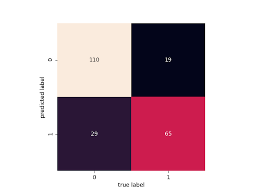
Now, we can see that the possibility of false positives is higher than false negatives.
Support Vector Machines
Support Vector Machines (SVMs) are robust, non-probabilistic models that can be used to predict both classification and regression problems. SVMs maximize space to widen the gap between categories and increase accuracy.
Let’s have a look:
from sklearn import svm

from base import Base


Xtrain, Xtest, ytrain, ytest = Base.clean_and_split()


model = svm.LinearSVC(random_state=800)

model.fit(Xtrain, ytrain)

ypred = model.predict(Xtest)


print("\n\nSVM Accuracy Score:", Base.accuracy_score(ytest, ypred), "%")
As you can see, SVMs are generally more accurate than other methods. If even better data cleansing methods are applied, we can aim to reach higher accuracy.
[Running] python -u "/top-10-machine-learning-algorithms-sklearn/svm.py"

SVM Accuracy Score: 79.0 %

[Done] exited with code=0 in 1.379 seconds
Now, instead of visualizing model data, let’s look at model performance. We can look at the classification report using scikit learn’s metrics module:
             precision    recall  f1-score   support


          0       0.85      0.82      0.83       144

          1       0.69      0.73      0.71        79


   accuracy                           0.79       223

  macro avg       0.77      0.78      0.77       223

weighted avg       0.79      0.79      0.79       223
Stochastic Gradient Descent Classification
Stochastic Gradient Descent (SGD) is popular in the neural network world, where it’s used to optimize the cost function. However, we can also use it to classify data. SGD is great for scenarios in which you have a large dataset with a very large feature set. It can help to reduce the complexities involved in learning from highly variable data.
from sklearn.linear_model import SGDClassifier

from base import Base


Xtrain, Xtest, ytrain, ytest = Base.clean_and_split()


model = SGDClassifier()

model.fit(Xtrain, ytrain)

ypred = model.predict(Xtest)


print("\n\nStochastic Gradient Descent Classifier Accuracy Score:", Base.accuracy_score(ytest, ypred), "%")
Let’s look at how accurate it is:
[Running] python -u "/top-10-machine-learning-algorithms-sklearn/stochastic_gradient_descent_classifier.py"


Stochastic Gradient Descent Classifier Accuracy Score: 76.0 %

[Done] exited with code=0 in 0.779 seconds
Logistic Regression
This is a very basic model that still delivers decent results. It’s a statistical model that uses logistic (sigmoid) functions to accurately predict data.
Before you use this model, you need to ensure that your training data is clean and has less noise. Significant variance could lower the accuracy of the model.
from sklearn.linear_model import LogisticRegression

from base import Base


Xtrain, Xtest, ytrain, ytest = Base.clean_and_split()


model = LogisticRegression()

model.fit(Xtrain, ytrain)

ypred = model.predict(Xtest)


print("\n\nLogistic Regression Accuracy Score:", Base.accuracy_score(ytest, ypred), "%")


=> Logistic Regression Accuracy Score: 79.0 %
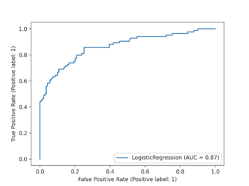
Now, let’s plot the Receiver Operating Characteristics (ROC) curve for this model. This curve helps us visualize accuracy by plotting the true positive rate on the Y axis and the false positive rate on the X axis. The “larger” the area under the curve, the more accurate the model.
Voting Classifier
Voting Classifier is another ensemble method where instead of using the same type of “weak” learners, we choose very different models. The idea is to combine conceptually different ML algorithms and use a majority vote to predict the class labels. This is useful for a set of equally well-performing models since it can balance out individual weaknesses.
For this ensemble, I will combine a Logistic Regression model, a Naive Bayes model, and a Random Forest model:
from sklearn.ensemble import VotingClassifier

from sklearn.linear_model import LogisticRegression

from sklearn.naive_bayes import GaussianNB

from sklearn.ensemble import RandomForestClassifier

from sklearn.model_selection import cross_val_score

from sklearn.model_selection import train_test_split

from base import Base


df = Base.clean()

X = df.drop(['Survived'], axis=1)

y = df['Survived']

Xtrain, Xtest, ytrain, ytest = train_test_split(X, y, random_state=0)


model_1 = LogisticRegression()

model_1.fit(Xtrain, ytrain)

ypred = model_1.predict(Xtest)


model_2 = GaussianNB()

model_2.fit(Xtrain, ytrain)

ypred = model_2.predict(Xtest)


model_3 = RandomForestClassifier()

model_3.fit(Xtrain, ytrain)

ypred = model_3.predict(Xtest)


eclf = VotingClassifier(

 estimators=[('lr', model_1), ('rf', model_2), ('gnb', model_3)],

 voting='hard'

)


for clf, label in zip([model_1, model_2, model_3, eclf], ['Logistic Regression', 'Naive Bayes', 'Random Forest', 'Ensemble']):

 scores = cross_val_score(clf, X, y, scoring='accuracy', cv=5)

 print("Accuracy: %0.2f (+/- %0.2f) [%s]" % (scores.mean(), scores.std(), label))
Let’s see how it performs:
[Running] python -u "/top-10-machine-learning-algorithms-sklearn/voting.py"


Accuracy: 0.79 (+/- 0.02) [Logistic Regression]

Accuracy: 0.78 (+/- 0.03) [Naive Bayes]

Accuracy: 0.80 (+/- 0.03) [Random Forest]

Accuracy: 0.80 (+/- 0.02) [Ensemble]


[Done] exited with code=0 in 2.413 seconds
As you can see, the Voting Ensemble learned from all three models and outperformed them all.
Conclusions: Right Algorithm for the Right Job
It is quite unfair to pit algorithms against each other. They’re all unique in their own way, and they all come with their own set of advantages and disadvantages. Before choosing which model works best for you, you should ensure that you understand the underlying dataset and feature set. Plot out variances and correlations before you try models out. If you’re still stuck after that, maybe the Voting Classifier can save your day.
- You can check out all of this code on GitHub.
- Download our Top 10 Algorithms Python environment, and try out the algorithms against your dataset to see how they perform.
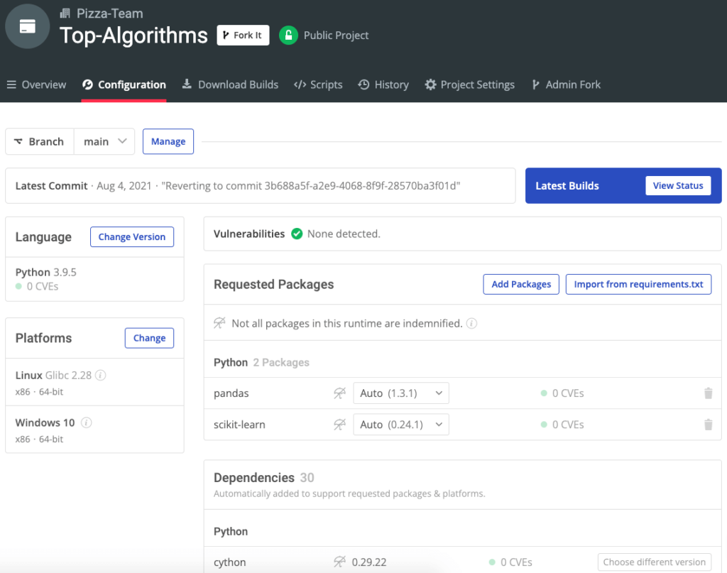
With the ActiveState Platform, you can create your Python environment in minutes, just like the one we built for this project.