Machine learning extracts patterns from data without explicit instructions.
Previously, we have discussed unsupervised learning methods, such as clustering1 and principal component analysis2, as well as supervised learning methods, such as random forests3, for classification and for predicting continuous outcomes. This month, we begin a series that looks more deeply into machine learning (ML) algorithms that extract patterns from data to generate insight4,5. In this primer, we will focus on essential ML principles. Future columns will explore the details of ML as well as its relationship to classical statistics.
ML is a modeling strategy to let the data speak for themselves, to the extent possible, which makes it an attractive option for characterizing and predicting complex biological phenomena that do not have a priori models. The benefits of ML arise from its use of a large number of tuning parameters or weights, which control the algorithm’s complexity and are estimated from the data using numerical optimization. ML algorithms are often motivated by heuristics such as models of interacting neurons or natural evolution—even if the underlying mechanism of the biological system being studied is substantially different from the heuristic model. The utility of ML algorithms is typically assessed empirically by determining how accurately and reliably extracted patterns generalize to new observations.
To show how ML can identify patterns, we will simulate a supervised learning scenario in which we want to predict the level of a hormone based on the concentration of a metabolite in the blood. Because the ground-truth relationship between the hormone and metabolite concentration is unknown, we will use ML to attempt to learn a close approximation from the data by simpler functions.
Suppose that the true relationship (target function) between the metabolite concentration (x) and the hormone level (y) is the 5th degree (d = 5) polynomial, y = x(x – 0.4)(x – 0.5)(x – 0.7)(x – 1), scaled appropriately so that both metabolite concentration and hormone level are in the range [0,1] (Fig. 1a). We use a polynomial because it is a familiar class of functions whose complexity (degree) is readily understood, not because it is a realistic target for a particular process.

We can reasonably approximate the polynomial target function with lower degree polynomials, which mimic the pattern in the studied relationship (Fig. 1a). Here, we have used a linear least-squares regression fit whose regression coefficients are the tuning parameters. The complexity of the fit is measured by the number of tuning parameters and is controlled by the degree of the polynomial. However, low-degree polynomials cannot approximate every pattern in data. If the target function were actually sinusoidal, approximating it with low-degree (e.g., d < 6) polynomials would be less successful and have larger error (Fig. 1b).
We can assess the quality of the approximation (ŷ) using the mean squared error (MSE = ∑(ŷi – yi)2/n). We obtain a low MSE when approximating the polynomial target with lower degree polynomials but a relatively large MSE when the target is a sinusoid (Fig. 1c). The success of any learning algorithm depends on whether there is a good match between the fitting functions and the target function. Since the target function is unknown, there is always a possibility that the data may exhibit relevant patterns beyond our model’s learning capabilities.
The fitting functions in our example had only a modest number of tuning parameters—the d = 5 polynomial had only six. To demonstrate learning with a large number of parameters and the impact of sample size and noise on the process, let’s increase the number of metabolites from one to five, (x1, x2, …, x5). We will use the same d = 5 degree polynomial as our target function; but instead of the concentration of a single metabolite, its output will be a function of the sum of the metabolites’ concentration, x =∑xi.
In this simple scenario, each of the five metabolites contributes equally. But, practically, we would not know that this is the case, nor would we know that the target function is a d = 5 degree polynomial. Thus, we would fit a function of all five metabolites, which would allow each to have its own weight in the fit. For example, if we fit the target with a d = 2 polynomial, we would be fitting to a constant term, linear terms (xi), pure quadratic terms (xi2) and the cross-product terms (xixj). A d = 3 polynomial fit would add pure cubic terms (xi3) and mixed terms (xi2xj, xixjxk). The d = 5 fit to all five metabolites has over 250 tuning parameters.
Let’s simulate a training set of 1,000 observations, from which we will attempt to learn the target function. Each observation will be a set of five metabolite concentrations sampled uniformly from the range [0,0.2] and the ground-truth value of the target, which is given by our d = 5 polynomial. To realistically reflect the presence of measurement error, we have added normal noise with mean zero and s.d. = 0.01 to metabolite and target in each observation. We will fit the observations, as we did for the noiseless case in Figure 1a, using polynomials of degree d = 1–5.
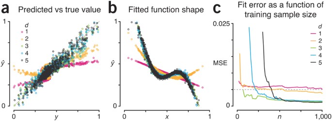
Figure 2a shows the profile of fitted versus target values (ŷ versus y) for each value of the fitting polynomial degree d using our simulated training set size of 1,000 observations. We come reasonably close to predicting the target function value around its average (0.43), but elsewhere our prediction is far off, in particular for low d. We can see the reason for this in Figure 2b, where we show our fitted approximation of the target function as a function of the sum of metabolite concentrations (like in Fig. 1a): low d polynomials are too simple to capture the bends in the target function.

We expect that as the training set size increases, noise will be mitigated, and our approximation will improve. However, for fits with d < 5, we expect the fit error to plateau—not only because of noise, but also because models with d < 5 are too simple to capture the complexity in the d = 5 target function.
Indeed, this is what we see when we plot the fit MSE as a function of training set size n (Fig. 2c). The MSE of the simplest d = 1 model plateaus quickly but is largest (0.0049) at n = 1,000. The MSE for the d = 3 fit is lower (0.0012), and the MSE for d = 5 is lower still (0.00096), but only marginally. We can also see that the learning process requires more samples to achieve the same MSE for models with higher complexity, because more tuning parameters must be estimated. For example, the d = 3, 4 and 5 fits reach MSE < 0.005 (dashed line, Fig. 2c) at n = 70, 220 and 410. The models with d = 1 and 2 take as long or longer to reach MSE = 0.005 because they plateau very close to this value.
In theory, if we knew all the inputs exactly, we could exactly predict the target function—identical metabolite profiles would have the same value of hormone level. In practice, there are always unknown inputs and imprecise measurements, so target function approximation has a random component, which varies from individual to individual. When there are many tuning parameters, it is easy to overfit by tuning to the noise in the training set6. This creates extra variability in the predictions on the test set and future observations.
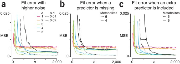
For example, if we were to continue sampling in Figure 2c, the MSE of the d = 5 fit would continue to drop, but it too would plateau eventually—in this case, not because the model wasn’t complex enough, but because of the noise in the system. Figure 3 demonstrates the effects of additional s.d. of the noise in the system on the quality of the fit. When we double the s.d of the noise from 0.01 to 0.02 (Fig. 3a), the MSE plateaus at a higher value. For example, the MSE for the d = 5 fit nearly quadruples from 0.0007 at n = 2,000 to 0.0027 (black arrow, Fig. 3a).

Let’s see what happens in the usual case that we do not know which of the metabolites are predictive of the target function. For example, if we do not include all of the actual metabolite concentrations used to calculate the target function, the effect of the unobserved metabolites appears as additional noise. We show this in Figure 3b, where the fit is performed with only four metabolites instead of five. The behavior of the MSE profiles is similar to Figure 3a: the MSE plateau is higher. In fact, failing to account for one of the predictor metabolites raises the d = 5 fit MSE plateau to 0.0039 (black arrow, Fig. 3b), which is even higher than when the s.d. of the noise was doubled as shown in Figure 3a.
Just as we may miss a predictor, we may overestimate the number of metabolites that impact the target function. In this case, however, we can reach the same MSE as with the right number of predictors but require a larger sample to do so. We show this in Figure 3c, where the fits are now performed with six metabolites instead of five. The d = 5 MSE eventually plateaus at 0.0007, just as in Figure 2b, but it does so more slowly. For example, the number of samples required for the d = 5 fit to reach MSE = 0.01 increases from n = 380 to 650 when an extraneous metabolite is included (black arrow, Fig. 3c).
ML is flexible in discovering patterns in data and, with sufficient observations, complex relationships can be approximated reasonably well. However, we must exercise judgment when selecting our model and predictors, otherwise our approximation may never be accurate.