Machine learning (ML) models can be astonishingly good at making predictions, but they often can’t yield explanations for their forecasts in terms that humans can easily understand. The features from which they draw conclusions can be so numerous, and their calculations so complex, that researchers can find it impossible to establish exactly why an algorithm produces the answers it does.
It is possible, however, to determine how a machine learning algorithm arrived at its conclusions.
This ability, otherwise known as “interpretability,” is a very active area of investigation among AI researchers in both academia and industry. It differs slightly from “explainability”–answering why–in that it can reveal causes and effects of changes within a model, even if the model’s internal workings remain opaque.
Interpretability is crucial for several reasons. If researchers don’t understand how a model works, they can have difficulty transferring learnings into a broader knowledge base, for example. Similarly, interpretability is essential for guarding against embedded bias or debugging an algorithm. It also helps researchers measure the effects of trade-offs in a model. More broadly, as algorithms play an increasingly important role in society, understanding precisely how they come up with their answers will only become more critical.
Researchers currently must compensate for incomplete interpretability with judgement, experience, observation, monitoring, and diligent risk management–including a thorough understanding of the datasets they use. However, several techniques exist for enhancing the degree of interpretability in machine learning models, regardless of their type. This article summarizes several of the most common of these, including their relative advantages and disadvantages.
Interpretable ML models and “Black Boxes”
Some machine learning models are interpretable by themselves. For example, for a linear model, the predicted outcome Y is a weighted sum of its features X. You can visualize “y equals a X plus b” in a plot as a straight line: a, the feature weight, is the slope of the line, and b is the intercept of the y-axis.
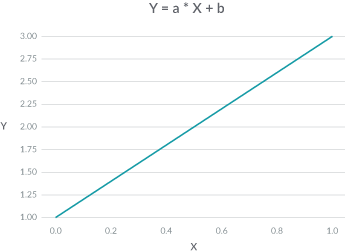
Linear models are user-friendly because they are simple and easy to understand. However, achieving the highest accuracy for large modern datasets often requires more complex and expressive models, like neural networks.
The following image shows a small, fully connected neural network, one of the simplest neural architectures. But even for this simplest neural architecture, there’s no way for anyone to understand which neuron is playing what role, and which input feature actually contributes to the model output. For this reason, such models are sometimes called “black boxes.”
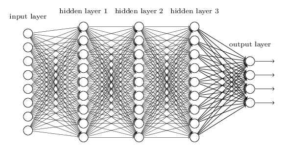
Now imagine a model with millions of neurons, and all sorts of connections. Without robust interpretability techniques, it would be difficult for a researcher to understand it at all.
Model-agnostic interpretability methods
Several important model-agnostic interpretability methods exist, and while none of them are perfect, they can help researchers interpret the results of even very complex ML models.
For demonstration purposes, let’s consider a small time-series dataset. A time series is simply a series of data points indexed in time order. It is the most common type of data in the financial industry. A frequent goal of quantitative research is to identify trends, seasonal variations, and correlation in financial time series data using statistical and machine learning methods.
Problem
- Data:
- Time series data (X, y)
- Model:
- model = RandomForestRegressor (n_estimators=10, max_depth=3)
- model.fit (X, y)
- Prediction:
- ŷ = model.predict (X)
The model used in this example is a RandomForestRegressor from sklearn.
Method 1: Partial Dependence Plot (PDP)
The first method we’ll examine is Partial Dependence Plot or PDP, which was invented decades ago, and shows the marginal effect that one or two features have on the predicted outcome of a machine learning model.
It helps researchers determine what happens to model predictions as various features are adjusted.
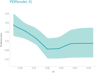
Here in this plot, the x-axis represents the value of feature f0, and the y-axis represents the predicted value. The solid line in the shaded area shows how the average prediction varies as the value of f0 changes.
PDP is very intuitive and easy to implement, but because it only shows the average marginal effects, heterogeneous effects might be hidden.1 For example, one feature might show a positive relationship with prediction for half of the data, but a negative relationship for the other half. The plot of the PDP will simply be a horizontal line.
To solve this problem, a new method was developed.
Method 2: Individual Conditional Expectation (ICE)
Individual Conditional Expectation or ICE, is very similar to PDP, but instead of plotting an average, ICE displays one line per instance.
This method is more intuitive than PDP because each line represents the predictions for one instance if one varies the feature of interest.
Like partial dependence, ICE helps explain what happens to the predictions of the model as a particular feature varies.
ICE displays one line per instance:
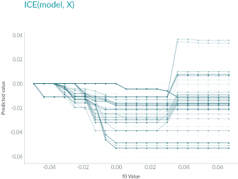
Unlike PDP, ICE curves can uncover heterogeneous relationships. However, this benefit also comes with a cost: it might not be as easy to see the average effect as it is with PDP.
Method 3: Permuted Feature Importance
Permuted Feature Importance is another traditional interpretability method.
The importance of a feature is the increase in the model prediction error after the feature’s values are shuffled. In other words, it helps define how the features in a model contribute to the predictions it makes.
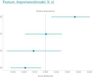
In the plot below, the x-axis represents the score reduction, or model error, and the y-axis represent each feature f0, f1, f2, f3.
As the plot shows, feature f2, the feature on top, has the largest impact on the model error; while f1, the second feature from the top, has no impact on the error after the shuffling. The remaining two features have negative contributions to the model.
PDP vs. ICE vs. Feature Importance
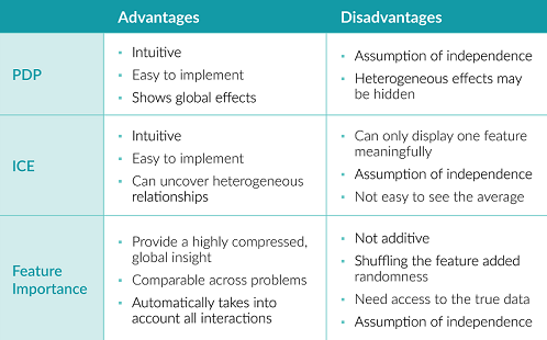
All three of the methods above are intuitive and easy to implement.
PDP shows global effects, while hiding heterogeneous effects. ICE can uncover heterogeneous effects, but makes it hard to see the average.
Feature importance provides a concise way to understand the model’s behavior. The use of error ratio (instead of the error) makes the measurements comparable across different problems. And it automatically takes into account all interactions with other features.
However, the interactions are not additive. Adding up feature importance does not result in a total drop in performance. Shuffling the features adds randomness, so the results may be different each time. Also, the shuffling requires access to true outcomes, which is impossible for many scenarios.
Besides, all three methods assume the independence of the features, so if features are correlated, unlikely data points will be created and the interpretation can be biased by these unrealistic data points.
Method 4: Global Surrogate
The global surrogate method takes a different approach. In this case, an interpretable model is trained to approximate the prediction of a black box model.
The process is simple. First you get predictions on a dataset with the trained black box model, and then train an interpretable model on this dataset and predictions. The trained interpretable model now becomes a surrogate of the original model, and all we need to do is to interpret the surrogate model. Note, the surrogate model could be any interpretable model: linear model, decision tree, human defined rules, etc.
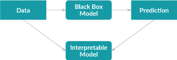
Using an interpretable model to approximate the black box model introduces additional error, but the additional error can easily be measured by R-squared.
However, since the surrogate models are only trained on the predictions of the black box model instead of the real outcome, global surrogate models can only interpret the black box model, but not the data.
Method 5: Local Surrogate (LIME)
Local Surrogate, or LIME (for Local Interpretable Model-agnostic Explanations), is different from global surrogate, in that it does not try to explain the whole model. Instead, it trains interpretable models to approximate the individual predictions.
LIME tries to understand how the predictions change when we perturb the data samples. Here is an example of LIME explaining why this picture is classified as a tree frog by the model.
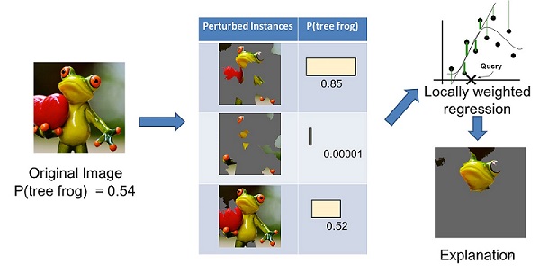
First the image on the left is divided into interpretable components. LIME then generates a dataset of perturbed instances by turning some of the interpretable components “off” (in this case, making them gray).
For each perturbed instance, one can use the trained model to get the probability that a tree frog is in the image, and then learn a locally weighted linear model on this dataset.
In the end, the components with the highest positive weights are presented as an explanation.
Global vs. Local Surrogate Methods
Both the global and local surrogate methods have advantages and disadvantages.
Global surrogate cares about explaining the whole logic of the model, while local surrogate is only interested in understanding specific predictions.
With the global surrogate method, any interpretable model can be used as surrogate, and the closeness of the surrogate models to the black box models can easily be measured.
However, since the surrogate models are trained only on the predictions of the black box model instead of the real outcome, they can only interpret the model, and not the data. Besides, the surrogate models, which are simpler than the black box model in a lot of cases, may only be able to give good explanations to part of the data, instead of the entire dataset.
The local surrogate method, on the other hand, does not share these shortcomings. In addition, the local surrogate method is model-agnostic: If you need to try a different black box model for your problem, you can still use the same surrogate models for interpretations. And compared with interpretations given by global surrogate methods, the interpretations from local surrogate methods are often short, contrastive, and human-friendly.
However, local surrogate has its own issues.
First, LIME uses a kernel to define the area within which data points are considered for local explanations, but it is difficult to find the proper kernel setting for a task. The way sampling is done in LIME can lead to unrealistic data points, and the local interpretation can be biased towards those data points.
Another concern is the instability of the explanations. Two very close points could lead to two very different explanations.
Method 6: Shapley Value (SHAP)
The concepts underlying Shapley Value, come from game theory. In this method, a prediction can be explained by assuming that each feature value of the instance is a “player” in a game. The contribution of each player is measured by adding and removing the player from all subsets of the rest of the players. The Shapley Value for one player is the weighted sum of all its contributions.
Shapley Value is additive and locally accurate. If you add up the Shapley Values of all the features, plus the base value, which is the prediction average, you will get the exact prediction value. This is a feature that many other methods do not have.
Here is an example from github. The experiment attempts to predict house prices with 13 features using the Xgboost model.

The plot shows the Shapley Value of each feature, representing the contribution that pushes the model outcome from base value to the final prediction. The red color means a positive contribution, and the blue color means a negative contribution.
The plot shows that, in this dataset, a feature called LSTAT (% lower status of the population, based on educational attainment and occupation) has the most impact on the prediction, and a high LSTAT lowers the predicted home price.2
Shapley Value vs. LIME
As data scientist Christoph Molnar points out in Interpretable Machine Learning, the Shapley Value might be the only method to deliver a full interpretation, and it is the explanation method with the strongest theoretical basis.
There are, however, trade-offs. Calculating the Shapley Value is computationally expensive. The recently developed kernel SHAP method does a fast kernel approximation to solve this problem, but for large background data, it still costs a lot of computation.
Unlike LIME, the Shapley Value does not return a prediction model. Finally, calculating the the Shapley Value for a new data instance requires access to the real data, not simply the prediction function.
How to Pick the “Right” Interpretability Tool?
The table below summarizes the methods covered in this article, ordered from least to greatest complexity.3
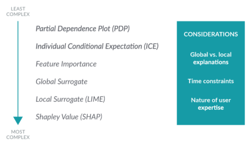
How should a researcher decide which method is the best for a given problem? Keep the following three considerations in mind:
- Do you need to understand the whole logic of a model, or do you only care about the reasons for a specific decision? That will help you decide whether you want a global method or local method.
- What’s your time limitation? If the user needs to quickly take a decision (e.g., a natural disaster may be imminent and public officials have to evaluate possible responses), it may be preferable to have an explanation that is simple to understand. But if the decision time is not a constraint (e.g., during a procedure to release a loan) one might prefer a more complex and exhaustive explanation.
- What is the user’s expertise level? Users of a predictive model may have different background knowledge and experience in the task. They can be decision-makers, scientists, engineers, etc. Knowing the user experience in the task is a key aspect of the perception of interpretability of a model. Domain experts may prefer a more sophisticated interpretation while others might want one that is easy to understand and remember.
Having decided which method best meets one’s needs, how can researchers evaluate an interpretation on our data or tasks?
Interpretability Evaluation Methods
There are currently three major ways to evaluate interpretability methods: application-grounded, human-grounded, and functionally grounded.
- Application-grounded evaluation requires a human to perform experiments within a real-life application.4 For example, to evaluate an interpretation on diagnosing a certain disease, the best way is for the doctor to perform diagnoses.
- Human-grounded evaluation is about conducting simpler human-subject experiments. For example, humans are presented with pairs of explanations, and must choose the one that they find to be of higher quality.
- Functionally grounded evaluation requires no human experiments. Instead, it uses a proxy for explanation quality. This method is much less costly than the previous two. The challenge, of course, is to determine what proxies to use. For example, decision trees have been considered interpretable in many situations, but additional research is required.
Summing Up
Interpretability remains a very active area of research in machine learning, and for good reason. The major model-agnostic methods surveyed in this post each represent a step toward more fully understanding machine learning models. As machine learning becomes more and more ubiquitous, grasping how these models find answers will be crucial to improving their performance and reliability.