- Introduction To Ensemble Learning
- Ensemble Learning Methods
- Bagging
- What is Bagging? How it works?
- Bagging
- Boosting
- What is Boosting?
- How Adaboost Algorithm Works?
- Other Boosting Algorithms
- Conclusion Ensemble Learning
- Project on Ensemble Learning
Introduction To Ensemble Learning
Ensemble Learning Techniques in Machine Learning, Machine learning models suffer bias and/or variance. Bias is the difference between the predicted value and actual value by the model. Bias is introduced when the model doesn’t consider the variation of data and creates a simple model. The simple model doesn’t follow the patterns of data, and hence the model gives errors in predicting training as well as testing data i.e. the model with high bias and high variance. You Can also read Covariance and Correlation In Machine Learning
When the model follows even random quirks of data, as pattern of data, then the model might do very well on training dataset i.e. it gives low bias, but it fails on test data and gives high variance.
Therefore, to improve the accuracy (estimate) of the model, ensemble learning methods are developed. Ensemble is a machine learning concept, in which several models are trained using machine learning algorithms. It combines low performing classifiers (also called as weak learners or base learner) and combine individual model prediction for the final prediction.
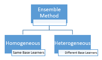
On the basis of type of base learners, ensemble methods can be categorized as homogeneous and heterogeneous ensemble methods. If base learners are same, then it is a homogeneous ensemble method. If base learners are different then it is a heterogeneous ensemble method.
Ensemble Learning Methods
Ensemble techniques are classified into three types:
- Bagging
- Boosting
- Stacking
Bagging
Consider a scenario where you are looking at the users’ ratings for a product. Instead of approving one user’s good/bad rating, we consider average rating given to the product. With average rating, we can be considerably sure of quality of the product. Bagging makes use of this principle. Instead of depending on one model, it runs the data through multiple models in parallel, and average them out as model’s final output.
What is Bagging? How it works?
- Bagging is an acronym for Bootstrapped Aggregation. Bootstrapping means random selection of records with replacement from the training dataset. ‘Random selection with replacement’ can be explained as follows:
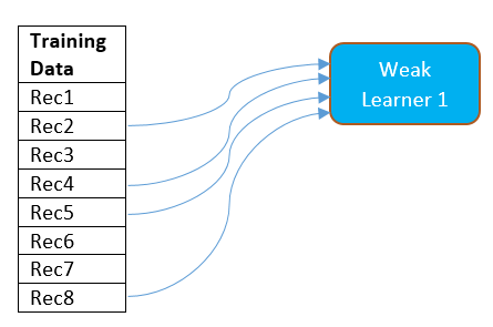
- Consider that there are 8 samples in the training dataset. Out of these 8 samples, every weak learner gets 5 samples as training data for the model. These 5 samples need not be unique, or non-repetitive.
- The model (weak learner) is allowed to get a sample multiple times. For example, as shown in the figure, Rec5 is selected 2 times by the model. Therefore, weak learner1 gets Rec2, Rec5, Rec8, Rec5, Rec4 as training data.
- All the samples are available for selection to next weak learners. Thus all 8 samples will be available for next weak learner and any sample can be selected multiple times by next weak learners.
- Bagging is a parallel method, which means several weak learners learn the data pattern independently and simultaneously. This can be best shown in the below diagram:

- The output of each weak learner is averaged to generate final output of the model.
- Since the weak learner’s outputs are averaged, this mechanism helps to reduce variance or variability in the predictions. However, it does not help to reduce bias of the model.
- Since final prediction is an average of output of each weak learner, it means that each weak learner has equal say or weight in the final output.
To summarize:
- Bagging is Bootstrapped Aggregation
- It is Parallel method
- Final output is calculated by averaging the outputs produced by individual weak learner
- Each weak learner has equal say
- Bagging reduces variance
Boosting
We saw that in bagging every model is given equal preference, but if one model predicts data more correctly than the other, then higher weightage should be given to this model over the other. Also, the model should attempt to reduce bias. These concepts are applied in the second ensemble method that we are going to learn, that is Boosting.
What is Boosting?
- To start with, boosting assigns equal weights to all data points as all points are equally important in the beginning. For example, if a training dataset has N samples, it assigns weight = 1/N to each sample.
- The weak learner classifies the data. The weak classifier classifies some samples correctly, while making mistake in classifying others.
- After classification, sample weights are changed. Weight of correctly classified sample is reduced, and weight of incorrectly classified sample is increased. Then the next weak classifier is run.
- This process continues until model as a whole gives strong predictions.
Note: Adaboost is the ensemble learning method used in binary classification only.
How Adaboost Algorithm Works?
Consider below training data for heart disease classification.

1. Initialize Weights To All Training Points
First step is to assign equal weights to all samples as all samples are equally important. Always, sum of weights of all samples equals 1. There are 8 samples, so each sample will get weight = 1/8 = 0.125
Since all samples are equally important to start with, all samples get equal weight: 1 / total number of samples = 1/8

2. Create Stump
After assigning weight, next step is to create stumps. Stump is a decision tree with one node and two leaves. Adaboost creates forest of decision stumps. To create stump, only one attribute should be chosen. But, it is not randomly selected. The attribute that does the best job of classifying the sample is selected first.
So let’s see how each attribute classifies the samples.
Blocked Artery:

Chest Pain:

Weight:
Weight is continuous quantity, and there is a method to find threshold for continuous quantity in decision tree algorithm. According to that method, the threshold is 175. Based on this condition draw the decision stump.

From above classification, it can be seen that
- ‘Blocked Arteries’ as a stump made 4 errors.
- ‘Chest Pain’ as a stump made 3 errors.
- ‘Weight’ as a stump made 1 error.
Since, the attribute ‘Weight’ made least number of errors, ‘Weight’ is the best stump to start with.
Note: Since this was attribute selection for first stump, we need not consider weight of each sample. This is because, to start with, all samples have equal weights.
To select next stump, both, weight of samples and errors made by that attribute while classifying the samples, will be considered.
3. Calculate Total Error And Voting Power (Amount Of Say) Of The Stump
After choosing best attribute for stump, next step is to calculate the voting power (amount of say) of that stump in the final classification. Formula to calculate amount of say is:

Where ln is Natural Log
Total Error = Number of misclassified samples * Weight of sample.
Since the stump misclassified only 1 sample, Total Error made by stump = weight of 1 sample = 1/8 = 0.125
Substituting Total Error in the equation,
Amount of say = ½ * ln((1-0.125)/0.125)
= 0.9729
4. Start To Build Final Classifier Function
The Adaboost classifier then starts building a function that will assign this ‘amount of say’ as voting power of the stump. It will assign 0.9729 as voting power to the stump created for ‘Weight’ attribute.
The function h(x) = 0.9729* ‘Weight’ as stump
5. Update New Weights For The Classifier
After calculation of amount of say, next step is to create another stump. However, before that adjust the weights assigned to each sample. The samples that were correctly classified in previous stump should get less importance as their classification is over, and the samples that were not correctly classified should get more weight in the next step.
The formula to assign new weight for correctly classified samples is:

The formula to assign new weight for incorrectly classified samples is:

New weights of correctly classified samples =
Wnew = (0.128) / 2(1-0.125) = 0.07
New weights of incorrectly classified samples =
Wnew = (0.125) / (2*0.125) = 0.5
Substitute new weights:

From above classification, it can be seen that
- ‘Blocked Arteries’ as a stump made 4 errors. Therefore, Total Error for ‘Blocked Arteries’ = 0.07*4 = 0.28
- ‘Chest Pain’ as a stump made 3 errors. Therefore, Total Error for ‘Chest Pain’ = 0.07*3 = 0.21
- ‘Weight’ as a stump made 1 error. Therefore, Total error for weight = 1*0.5 = 0.5.
Note: We have already considered ‘Weight’ attribute for first stump creation. So this attribute need not be considered again. However, it is considered here to show effect of ‘Assigned Weight’ of the sample on Total Error calculation.
6. Calculate Voting Power (Amount of Say) and Add to Final Classifier Function
Since Chest Pain classifier has least Total Error, this attribute is selected as second stump.
The Amount of Say = ½ ln(1-0.21)/0.21 =0.66
Add this classifier with its weight to the function.
The function h(x) = 0.9729* ‘Weight’ as stump + 0.66*’Chest Pain’ as stump
7. Assign New Weights and Repeat
Again, assign new weights to the correctly classified samples with formula:
Wnew = Wold / 2(1-total weight)
And incorrectly classified samples with the formula:
Wnew = Wold / (2*total weight)
We repeat this process until
- Enough rounds of this process are done to create strong classifier
- No good classifiers left for making predictions.
When it comes to classifying data point, even if one classifier misclassifies a point, the voting powers of other classifiers override it making strong predictions.
There is another method to train Adaboost algorithm. In this method, new sample dataset is created in every iteration. The sample dataset is of same size as original dataset, and it contains some samples that are repeatedly selected. Samples with higher weights (i.e. samples that are incorrectly classified in previous round), will be selected repeatedly. The weight vector is normalized.
To summarize:
- Adaboost is a sequential method where one weak learner runs after other.
- Weak learners are stumps i.e. decision tree with 2 nodes.
- Voting power is assigned to stumps based on how correctly it classifies the data.
- Boosting reduces bias
Other Boosting Algorithms
Apart from Adaboost, there is other boosting algorithm – Gradient Boosting or Gradient Boosting Machine (GBM). The main idea behind this algorithm is to create decision trees with smaller leaves and scale the tree with a learning rate.
Decision tree algorithm is prone to overfitting and leads to high variance. Hence prediction made by the tree is scaled (or multipled) with the learning rate. This reduces training accuracy, but provides better results in long run. Gradient Boosting is used in classification as well as regression problems.
The open source implementations Gradient Boosting algorithms are XGBoost, LightGBM that are more regularized, and efficient.
Conclusion Ensemble Learning
In this article, we learned that Ensemble Learning Techniques in Machine Learning is used to improve the performance of the model. In this method, several models are combined and the prediction of each model is considered in the overall prediction.
Bagging and Boosting are ensemble methods. Bagging is Bootstrapped Aggregation and it is a parallel method. That means multiple models run in parallel and final output is calculated by averaging the outputs produced by individual model. In Bagging, each weak learner has equal say in final output prediction. Bagging reduces the variance.
Boosting is a sequential method where mistakes made by first weak learner are considered while making predictions by second weak learner. Weights are assigned and adjusted in each iteration. Boosting reduces bias. Adaboost, GBM, LightGBM are some of the boosting techniques used to improve overall prediction of the model.