Semi-supervised learning (mixture of “labeled” and “unlabeled” data).
Reinforcement learning. Using this algorithm, the machine is trained to make specific decisions. It works this way: the machine is exposed to an environment where it trains itself continually using trial and error. This machine learns from past experience and tries to capture the best possible knowledge to make accurate business decisions. Example of Reinforcement Learning: Markov Decision Process.
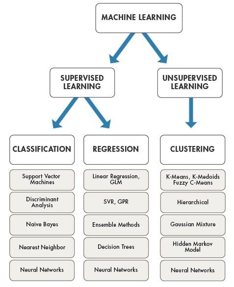
There are lots of overlaps in which ML algorithms are applied to a particular problem. As a result, for the same problem, there could be many different ML models possible. So, coming out with the best ML model is an art that requires a lot of patience and trial and error. Following figure provides a brief of all these learning types with sample use cases.
The supervised learning algorithms are a subset of the family of machine learning algorithms which are mainly used in predictive modeling. A predictive model is basically a model constructed from a machine learning algorithm and features or attributes from training data such that we can predict a value using the other values obtained from the input data. Supervised learning algorithms try to model relationships and dependencies between the target prediction output and the input features such that we can predict the output values for new data based on those relationships which it learned from the previous data sets. The main types of supervised learning algorithms include:
Classification algorithms: These algorithms build predictive models from training data which have features and class labels. These predictive models in-turn use the features learnt from training data on new, previously unseen data to predict their class labels. The output classes are discrete. Types of classification algorithms include decision trees, random forests, support vector machines, and many more.
Regression algorithms: These algorithms are used to predict output values based on some input features obtained from the data. To do this, the algorithm builds a model based on features and output values of the training data and this model is used to predict values for new data. The output values in this case are continuous and not discrete. Types of regression algorithms include linear regression, multivariate regression, regression trees, and lasso regression, among many others.
Some application of supervised learning are speech recognition, credit scoring, medical imaging, and search engines.
The unsupervised learning algorithms are the family of machine learning algorithms which are mainly used in pattern detection and descriptive modeling. However, there are no output categories or labels here based on which the algorithm can try to model relationships. These algorithms try to use techniques on the input data to mine for rules, detect patterns, and summarize and group the data points which help in deriving meaningful insights and describe the data better to the users. The main types of unsupervised learning algorithms include:
Clustering algorithms: The main objective of these algorithms is to cluster or group input data points into different classes or categories using just the features derived from the input data alone and no other external information. Unlike classification, the output labels are not known beforehand in clustering. There are different approaches to build clustering models, such as by using means, medoids, hierarchies, and many more. Some popular clustering algorithms include k-means, k-medoids, and hierarchical clustering.
Association rule learning algorithms: These algorithms are used to mine and extract rules and patterns from data sets. These rules explain relationships between different variables and attributes, and also depict frequent item sets and patterns which occur in the data. These rules in turn help discover useful insights for any business or organization from their huge data repositories. Popular algorithms include Apriori and FP Growth.
Some applications of unsupervised learning are customer segmentation in marketing, social network analysis, image segmentation, climatology, and many more.
Semi-Supervised Learning. In the previous two types, either there are no labels for all the observation in the dataset or labels are present for all the observations. Semi-supervised learning falls in between these two. In many practical situations, the cost to label is quite high, since it requires skilled human experts to do that. So, in the absence of labels in the majority of the observations but present in few, semi-supervised algorithms are the best candidates for the model building. These methods exploit the idea that even though the group memberships of the unlabeled data are unknown, this data carries important information about the group parameters.
The reinforcement learning method aims at using observations gathered from the interaction with the environment to take actions that would maximize the reward or minimize the risk. Reinforcement learning algorithm (called the agent) continuously learns from the environment in an iterative fashion. In the process, the agent learns from its experiences of the environment until it explores the full range of possible states.
In order to produce intelligent programs (also called agents), reinforcement learning goes through the following steps:
Input state is observed by the agent.
Decision making function is used to make the agent perform an action.
After the action is performed, the agent receives reward or reinforcement from the environment.
The state-action pair information about the reward is stored.
Some applications of the reinforcement learning algorithms are computer played board games (Chess, Go), robotic hands, and self-driving cars.
Predictive model
A predictive model is used for tasks that involve the prediction of one value using other values in the dataset. The learning algorithm attempts to discover and model the relationship between the target feature (the feature being predicted) and the other features. Despite the common use of the word “prediction” to imply forecasting, predictive models need not necessarily foresee events in the future. For instance, a predictive model could be used to predict past events, such as the date of a baby’s conception using the mother’s present-day hormone levels. Predictive models can also be used in real time to control traffic lights during rush hours.
Because predictive models are given clear instruction on what they need to learn and how they are intended to learn it, the process of training a predictive model is known as supervised learning. The supervision does not refer to human involvement, but rather to the fact that the target values provide a way for the learner to know how well it has learned the desired task. Stated more formally, given a set of data, a supervised learning algorithm attempts to optimize a function (the model) to find the combination of feature values that result in the target output.
So, supervised learning consist of a target / outcome variable (or dependent variable) which is to be predicted from a given set of predictors (independent variables). Using these set of variables, we generate a function that map inputs to desired outputs. The training process continues until the model achieves a desired level of accuracy on the training data. Examples of Supervised Learning: Regression, Decision Tree, Random Forest, KNN, Logistic Regression etc.
The often used supervised machine learning task of predicting which category an example belongs to is known as classification. It is easy to think of potential uses for a classifier. For instance, you could predict whether:
An e-mail message is spam
A person has cancer
A football team will win or lose
An applicant will default on a loan
In classification, the target feature to be predicted is a categorical feature known as the class, and is divided into categories called levels. A class can have two or more levels, and the levels may or may not be ordinal. Because classification is so widely used in machine learning, there are many types of classification algorithms, with strengths and weaknesses suited for different types of input data.
Supervised learners can also be used to predict numeric data such as income, laboratory values, test scores, or counts of items. To predict such numeric values, a common form of numeric prediction fits linear regression models to the input data. Although regression models are not the only type of numeric models, they are, by far, the most widely used. Regression methods are widely used for forecasting, as they quantify in exact terms the association between inputs and the target, including both, the magnitude and uncertainty of the relationship.
Descriptive model
A descriptive model is used for tasks that would benefit from the insight gained from summarizing data in new and interesting ways. As opposed to predictive models that predict a target of interest, in a descriptive model, no single feature is more important than any other. In fact, because there is no target to learn, the process of training a descriptive model is called unsupervised learning. Although it can be more difficult to think of applications for descriptive models, what good is a learner that isn’t learning anything in particular – they are used quite regularly for data mining.
So, in unsupervised learning algorithm, we do not have any target or outcome variable to predict / estimate. It is used for clustering population in different groups, which is widely used for segmenting customers in different groups for specific intervention. Examples of Unsupervised Learning: Apriori algorithm, K-means.
For example, the descriptive modeling task called pattern discovery is used to identify useful associations within data. Pattern discovery is often used for market basket analysis on retailers’ transactional purchase data. Here, the goal is to identify items that are frequently purchased together, such that the learned information can be used to refine marketing tactics. For instance, if a retailer learns that swimming trunks are commonly purchased at the same time as sunglasses, the retailer might reposition the items more closely in the store or run a promotion to “up-sell” customers on associated items.
The descriptive modeling task of dividing a dataset into homogeneous groups is called clustering. This is sometimes used for segmentation analysis that identifies groups of individuals with similar behavior or demographic information, so that advertising campaigns could be tailored for particular audiences. Although the machine is capable of identifying the clusters, human intervention is required to interpret them. For example, given five different clusters of shoppers at a grocery store, the marketing team will need to understand the differences among the groups in order to create a promotion that best suits each group.
Lastly, a class of machine learning algorithms known as meta-learners is not tied to a specific learning task, but is rather focused on learning how to learn more effectively. A meta-learning algorithm uses the result of some learnings to inform additional learning. This can be beneficial for very challenging problems or when a predictive algorithm’s performance needs to be as accurate as possible.
The following table lists only a fraction of the entire set of machine learning algorithms.
Model
Learning task
Supervised Learning Algorithms
Nearest Neighbor
Classification
Naive Bayes
Classification
Decision Trees
Classification
Classification Rule Learners
Classification
Linear Regression
Numeric prediction
Model Trees
Numeric prediction
Regression Trees
Neural Networks
Dual use
Support Vector Machines
Dual use
Unsupervised Learning Algorithms
Association Rules
Pattern detection
k-means clustering
Clustering
Meta-Learning Algorithms
Bagging
Dual use
Boosting
Dual use
Random Forests
Dual use
To begin applying machine learning to a real-world project, you will need to determine which of the four learning tasks your project represents: classification, numeric prediction, pattern detection, or clustering. The task will drive the choice of algorithm. For instance, if you are undertaking pattern detection, you are likely to employ association rules. Similarly, a clustering problem will likely utilize the k-means algorithm, and numeric prediction will utilize regression analysis or regression trees.
Torsten Hothorn maintains an exhaustive list of packages available in R for implementing machine learning algorithms.
Model evaluation
Whenever we are building a model, it needs to be tested and evaluated to ensure that it will not only work on trained data, but also on unseen data and can generate results with accuracy. A model should not generate a random result though some noise is permitted. If the model is not evaluated properly then the chances are that the result produced with unseen data is not accurate. Furthermore, model evaluation can help select the optimum model, which is more robust and can accurately predict responses for future subjects.
There are various ways by which a model can be evaluated:
Split test. In a split test, the dataset is divided into two parts, one is the training set and the other is test dataset. Once data is split the algorithm will use the training set and a model is created. The accuracy of a model is tested using the test dataset. The ratio of dividing the dataset in training and test can be decided on basis of the size of the dataset. It is fast and great when the dataset is of large size or the dataset is expensive. It can produce different result on how the dataset is divided into the training and test dataset. If the date set is divided in 80% as a training set and 20% as a test set, 60% as a training set and 40%, both will generate different results. We can go for multiple split tests, where the dataset is divided in different ratios and the result is found and compared for accuracy.
Cross validation. In cross validation, the dataset is divided in number of parts, for example, dividing the dataset in 10 parts. An algorithm is run on 9 subsets and holds one back for test. This process is repeated 10 times. Based on different results generated on each run, the accuracy is found. It is known as k-fold cross validation is where k is the number in which a dataset is divided. Selecting the k is very crucial here, which is dependent on the size of dataset.
Bootstrap. We start with some random samples from the dataset, and an algorithm is run on dataset. This process is repeated for n times until we have all covered the full dataset. In aggregate, the result provided in all repetition shows the model performance.
Leave One Out Cross Validation. As the name suggests, only one data point from the dataset is left out, an algorithm is run on the rest of the dataset and it is repeated for each point. As all points from the dataset are covered it is less biased, but it requires higher execution time if the dataset is large.
Model evaluation is a key step in any machine learning process. It is different for supervised and unsupervised models. In supervised models, predictions play a major role; whereas in unsupervised models, homogeneity within clusters and heterogeneity across clusters play a major role.
Some widely used model evaluation parameters for regression models (including cross validation) are as follows:
Coefficient of determination
Root mean squared error
Mean absolute error
Akaike or Bayesian information criterion
Some widely used model evaluation parameters for classification models (including cross validation) are as follows:
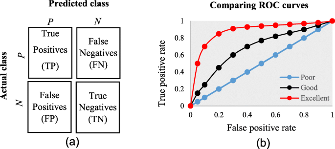
Confusion matrix (accuracy, precision, recall, and F1-score)
Gain or lift charts
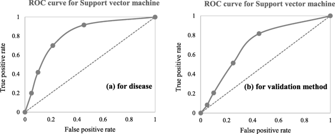
Area under ROC (receiver operating characteristic) curve
Concordant and discordant ratio
Some of the widely used evaluation parameters of unsupervised models (clustering) are as follows:
Contingency tables
Sum of squared errors between clustering objects and cluster centers or centroids
Silhouette value
Rand index
Matching index
Pairwise and adjusted pairwise precision and recall (primarily used in NLP)
Bias and variance are two key error components of any supervised model; their trade-off plays a vital role in model tuning and selection. Bias is due to incorrect assumptions made by a predictive model while learning outcomes, whereas variance is due to model rigidity toward the training dataset. In other words, higher bias leads to underfitting and higher variance leads to overfitting of models.
In bias, the assumptions are on target functional forms. Hence, this is dominant in parametric models such as linear regression, logistic regression, and linear discriminant analysis as their outcomes are a functional form of input variables.
Variance, on the other hand, shows how susceptible models are to change in datasets. Generally, target functional forms control variance. Hence, this is dominant in non-parametric models such as decision trees, support vector machines, and K-nearest neighbors as their outcomes are not directly afunctional form of input variables. In other words, the hyperparameters of non-parametric models can lead to overfitting of predictive models.
All machine learning fields—Supervised, Unsupervised, Semi-supervised, and Reinforcement learning, use several algorithms for different types of tasks like prediction, classification, regression, etc. Each machine learning algorithm handles one specific problem, and this way beginners can dive into one of these to figure out solutions, one at a time.
Here is a compilation of the top machine learning algorithms that are frequently used in all machine learning fields.
Now, you can practice ML algorithms here.
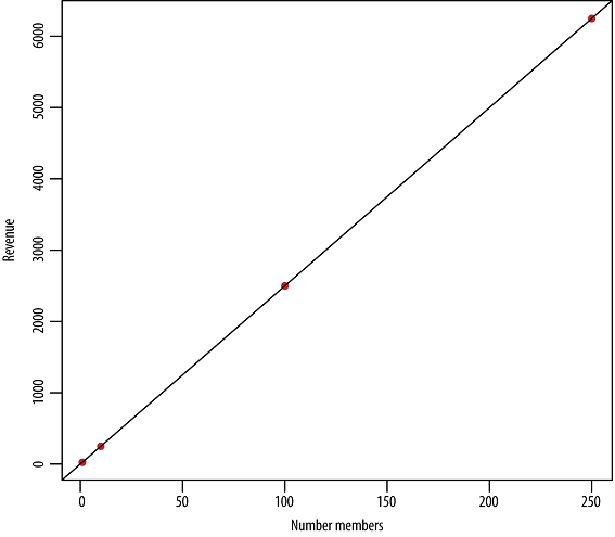
Linear regression
Forming relationships between two variables is almost the starting point of a model, and linear regression in machine learning achieves that. The relationship between the dependent and independent variables is established by aligning them on a regression line. Then, the objective is to find the best fit line that explains the relationship between both variables.
The linear regression line is represented by a mathematical equation by,
y = mx + c
Where y is the dependent variable, x is the independent variable, m is the slope, and c is the intercept.
Logistic regression
Now, when the dependent variable is dichotomous (binary), logistic regression is used to estimate the discrete values (unlike linear regression that handles continuous values) within a set of independent variables.
This algorithm is used in predictive analysis where probability of an event occurrence is predicted based on logit function, which is why it is also called ‘logit regression’.
Mathematically, it is represented by,
y = e^(b0 + b1*x) / (1 + e^(b0 + b1*x))
Where x is the input value, y is the predicted output, b0 is the bias, and b1 is the coefficient for x.
Artificial neural networks
ANNs are used in most of the recent AGI-related models that use self-supervised learning. This algorithm tries to mimic the human brain by copying the behaviour and connections of the neurons. The structure of ANNs has three or more layers that are interconnected for processing input data.
These are used in various smart appliances as well as automation devices like automatic cars, smart speakers and lights, and much more.
Convolutional neural networks (CNNs), one of the most used neural networks in recent developments, are a type of ANNs. These are mostly computer vision-based networks where the first layer is the input layer, the layers in between are the hidden layers that do that computing, and the third layer is the output layer.
Gradient descent
An optimisation algorithm for minimising cost function by updating parameters of the machine learning model. It is used inside various machine learning algorithms and is most commonly used in deep learning. It is used in various fields like robotics, computer games, mechanical engineering, and more.
There are three types of gradient descent algorithms:
Batch gradient descent: Processes all the training data for each iteration of gradient descent. If the dataset is large, this method is too expensive.
Stochastic gradient descent: This processes one training example per iteration, resulting in parameters getting updated every single time.
Mini batch gradient descent: The fastest gradient descent that processes large amounts of iterations in small batches, matching similar iterations.
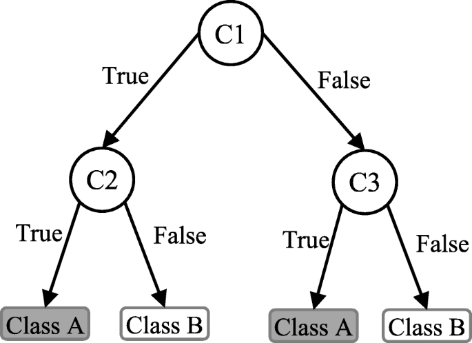
Decision trees
A supervised learning algorithm used for visualisation of a map of possible results for a series of decisions. Basically, it splits the dataset into two or more homogeneous for comparison of possible outcomes and then makes decisions based on advantages and probabilities.
It is like making a pros and cons list, and making decisions based on anticipations and potentiality of different options but, in machine learning, it is based on a mathematical construct.
Naive Bayes Algorithm
Bayesian probability is a type of probability concept where instead of frequency of a phenomenon, probability is interpreted by quantification of a personal belief or knowledge representing a reasonable expectation. The Naive Bayes is used for classification problems, and it assumes that features in the algorithm are independent of each other and are not impacted by changes in each other.
For example, the weight and size of a table can change and maybe interrelated but do not change the fundamental fact that it is a table. This simplistic algorithm is capable of handling large datasets and making predictions in real-time.
Bayes’ theorem is given by,
P (X|Y) = (P (Y|X) x P (X)) /P (Y)
Where P(X) is the probability of X being true, P(X/Y) is the conditional probability where X is true when Y is true as well.
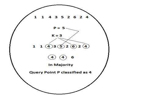
KNN Algorithm
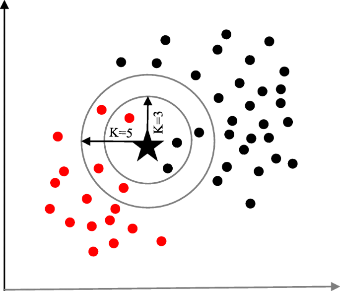
This supervised machine learning algorithm classifies all new cases based on old cases stored that are segregated into different classes based on their similarity scores. K Nearest Neighbours (KNN) is used for both regression and classification problems.
K refers to the number of nearby points considered during segregation and classification of a set of known groups. The algorithm does classification by a majority vote of the neighbouring K points.
Major use cases and real-life applications of the algorithm can be found in recommendation systems of OTT platforms like Amazon and Netflix, and also facial recognition systems.
K-Means
For clustering tasks, K-means is an unsupervised machine learning algorithm based on distance. The algorithm classifies datasets into K clusters where within one set, the data points remain homogenous, but not in different clusters.
This algorithm is used in clustering Facebook users who have common interests based on their likes and dislikes, and also segmentation of similar eCommerce products.
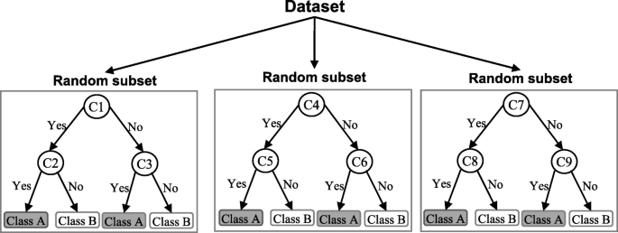
Random forest algorithm
Another supervised learning algorithm, Random trees is a collection of multiple decision trees that are built on different samples during training. It builds on the accuracy of decision trees by mapping decisions from different trees onto a single tree known as a CART model (Classification and Regression Trees).
This helps in increasing accuracy when in a dataset, a large chunk of data is missing. The final prediction is based on the prediction result which is voted the highest. This algorithm is mostly used in eCommerce recommendation engines and financial models.
Support Vector Machines
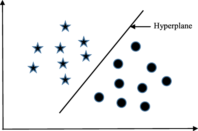
SVMs are supervised machine learning algorithms that plot individual data into a number of dimensional spaces, based on the number of features. Classification is performed by determining the hyper-plane that distincts two sets of support vectors.
Simply, SVMs are for representing coordinates of individual observations. These are popularly used in machine learning applications like facial expression classification, speech recognition, and image detection.
Machine learning and deep learning algorithms are all around us in modern businesses. The number of AI applications that may be used has been rapidly increasing with the rapid advancement of new algorithms, cheaper compute, and greater data availability. Every field, from banking to healthcare to education to manufacturing, construction, and beyond, has its own set of machine learning and deep learning solutions.
The biggest problem in all of these ML and DL projects across various sectors is model improvement. So, in this post, we’ll look at methods for improving machine learning models based on structured data (time-series, categorization) and deep learning models based on unstructured data (text, images, audio/video).
Importance of Data Structure
The first thing to understand before we get into strategies for machine learning modeling is to emphasize the importance of data i.e. “what kind of data do you have?”. This is important because ML requires a lot of data in order to train properly. This data must be organized in a way that is easy for the algorithm to understand and use. Data structures provide this organization, making machine learning possible. Without data structures, machine learning would be very difficult, if not impossible. Data must be carefully arranged so that the algorithm can learn from it effectively. Data structures provide this organization, allowing machine learning to take place.
As such, data can be classified into two categories:
Structured Data — is easier to process and analyze than unstructured data. It’s usually arranged in a fixed format that makes it easy to extract specific pieces of information, which can be helpful for certain types of predictions. For example, if you’re trying to predict how if the price of stock will go up in the next month, you might find it helpful to use data that’s been formatted as a table or spreadsheet. This type of data works best with supervised learning models.
Unstructured Data — can be a valuable source of information for predictions in machine learning, because it can contain more diverse and nuanced information than structured data. For example, unstructured text data can include information about the sentiment or emotional state of a customer, which might be useful for predicting whether that customer is likely to churn. This type of data works best with unsupervised learning models.
Table 1 — Structured & Unstructured Data Comparison
Machine Learning Algorithms Cheat Sheet
Information in this section provided by SAS Blog to be used for reference only.
Source: SAS Blog — ML Cheat Sheet
How to use the cheat sheet
Read the path and algorithm labels on the chart as “If <path label> then use <algorithm>.” For example:
If you want to perform dimension reduction then use principal component analysis.
If you need a numeric prediction quickly, use decision trees or linear regression.
If you need a hierarchical result, use hierarchical clustering.
Sometimes more than one branch will apply, and other times none of them will be a perfect match. It’s important to remember these paths are intended to be rule-of-thumb recommendations, so some of the recommendations are not exact. Several data scientists I talked with said that the only sure way to find the very best algorithm is to try all of them.
Strategies for Improving ML Models — Structured Data
There are many methods for improving machine learning models based on structured data. Some of the most common methods include:
1. Feature selection: Identifying and selecting the most relevant features from the data can help improve the accuracy of machine learning models. For example, selecting only the most important features from a dataset can help reduce overfitting and improve generalization.
2. Feature engineering: This involves transforming or creating new features from existing ones to better capture relationships in the data. For instance, one could engineer features that capture quadratic or cubic relationships between variables in order to improve the predictive power of a machine learning model.
3. Model selection and tuning: Trying out different machine learning models (e.g., linear regression, decision trees, random forests) and tuning their hyperparameters (e.g., regularization strength, tree depth) can help improve the performance of the final model.
4. Data pre-processing: This step can involve various techniques such as imputation (filling in missing values), outlier removal, and normalization/standardization. Proper data pre-processing can improve the accuracy of machine learning models.
Strategies for Improving ML Models — Unstructured Data
There are various methods for improving machine learning models based on unstructured data. Some of these methods include the following:
1. Using a pre-trained model: A pre-trained model is a machine learning model that has been trained on a large dataset, such as ImageNet. This type of model can be used to improve the performance of a machine learning model that is being trained on a smaller dataset.
2. Using more data: The more data that is available to train a machine learning model, the better the model will perform. This is because more data provides more opportunities for the algorithm to learn from and identify patterns in the data.
3. Training multiple models: Instead of training one single machine learning model, it can be beneficial to train multiple models. This is because each model can learn from different aspects of the data and improve the overall performance of the machine learning system.
4. Ensembling: Ensembling is a technique that combines the predictions of multiple machine learning models to produce a more accurate prediction. This can be done by training multiple models on the same dataset and then taking the average of their predictions, or by training multiple models on different subsets of the data and then taking the majority vote of their predictions.
5. Feature engineering: Feature engineering is the process of creating new features from existing data. This can be done by transforming existing features, such as using PCA to create new features from existing ones, or by creating new features from scratch, such as using the data from an accelerometer to create a new feature that represents the speed of the device.
6. Model tuning: Model tuning is the process of adjusting the hyperparameters of a machine learning model to improve its performance. This can be done by using techniques such as grid search or random search.
7. Regularization: Regularization is a technique that is used to prevent overfitting in machine learning models. This is done by adding constraints to the model, such as limiting the number of parameters that can be used, or by adding penalty terms to the objective function that are associated with large values of the parameters.
8. Data augmentation: Data augmentation is a technique that is used to generate new data from existing data. This can be done by randomly perturbing the existing data, such as adding noise to images or changing the order of words in text documents.
9. Transfer learning: Transfer learning is a technique that is used to learn from other tasks that are related to the task at hand. This can be done by pre-training a machine learning model on a large dataset and then fine-tuning it on the smaller dataset.
10. Dimensionality reduction: Dimensionality reduction is a technique that is used to reduce the number of features that are used to represent the data. The primary benefits of DR includes that it can help to simplify the data, making it easier to work with and understand, it can help to improve the results of machine learning algorithms by reducing the noise in the data and it can also reduce computational costs by reducing the number of features that need to be processed.
Strategies for Improving ML Models — Overall
There are many different ways to improve machine learning and deep learning models. Some common strategies include:
Using more data: This is often the most important factor in improving a model’s accuracy. The more data you can train your model on, the better it will perform.
Preprocessing the data: This can help improve the accuracy of your models by removing noise and spurious correlations from the data.
Manually tweaking the hyperparameters of your algorithms: This can help improve the performance of your models by optimizing them for your specific dataset and task.
Using ensembles of models: Combining multiple models into an ensemble can often lead to better performance than using a single model.
Normalization: Normalization is a technique used in machine learning to adjust the range of values in a dataset so that all values are within a certain range. This is often done to make sure that the data can be accurately processed by the machine learning algorithm. There are many different types of normalization, but usually it involves adjusting the data so that the mean value is zero and the standard deviation is one. This ensures that all values in the dataset are normalized within a range of -1 to 1.
Standardization: Standardization is a process of cleaning and preparing data so that it can be used in machine learning algorithms. This process involves rescaling variables so that they have a mean of 0 and a standard deviation of 1, which ensures that all the variables are in the same scale. Standardization is especially important when you are comparing different machine learning models, as it ensures that all the models are using the same data.
One-hot encoding: This technique transforms categorical variables into binary vectors. This is useful for datasets with features that are categorical (e.g., gender, race, etc.).
Understanding the errors: Machine learning models are only as good as the data they are trained on. If you don’t understand what kind of errors your AI model is making, you run the risk of perpetuating inaccurate information and biases. For example, if you have a machine learning model that is classifying images, and it is mistakenly classifying images of black people as gorillas, then you need to be aware of that error so you can fix it. Otherwise, your model will continue to incorrectly classify images, which could have serious implications for real-world applications.
Source: Tech eBay — The six phases of ML modeling and their acceptance criteria
Normalization of Data
Normalization is a machine learning technique that helps to standardize data so that it can be better processed by algorithms. By normalizing data, we can reduce the amount of variability in our dataset, making it more predictable and easier to work with. There are several different techniques for normalizing data, but the most common methods involve rescaling data so that all values lie between 0 and 1, or standardizing data so that each value has a mean of 0 and a standard deviation of 1.
One reason why Normalization is important is because many machine learning algorithms assume that data is normally distributed (i.e. bell-shaped). This means that if our data is not normalized, then these algorithms may not work as well. In addition, normalizing data can help to improve the accuracy of some machine learning algorithms, and can make it easier to compare different datasets.
When to Normalize Data?
Normalization is a feature scaling technique that is used when the data have an unknown distribution or do not have a Gaussian Distribution. This method of data scaling is employed when the data has a broad scope and the algorithms that train the data do not make assumptions about how it will be distributed, such as with an Artificial Neural Network.
Source: Analyst Answer
There are a few different ways to normalize data:
Source: Somenka.net
1. Rescaling: This means that all values in the dataset are scaled so that they lie between 0 and 1. To rescale data, we first need to calculate the minimum and maximum values for each feature (column). We then subtract the minimum value from each value in the column, and divide by the range (maximum — minimum).
· Tip: rescaling is a good choice if you want to ensure that all values in your dataset are between 0 and 1.
2. Standardization: This technique transforms data so that it has a mean of 0 and a standard deviation of 1. Unlike rescaling, standardization does not necessarily bound values to a specific range. To standardize data, we first need to calculate the mean and standard deviation for each column. We then subtract the mean from each value in the column, and divide by the standard deviation.
· Tip: Standardization is a good choice if you want to center your data around 0, or if you want to make sure that all values have the same scale.
3. Min-Max Scaling: This is a type of rescaling that transforms data so that all values lie between 0 and 1. Unlike other methods of rescaling, min-max scaling does not center the data around 0. Instead, it scales the data such that the minimum value is 0 and the maximum value is 1. To min-max scale data, we first need to calculate the minimum and maximum values for each column. We then subtract the minimum value from each value in the column, and divide by the range (maximum — minimum).
· Tip: Min-Max Scaling is a good choice if you want to ensure that all values in your dataset are between 0 and 1, but you don’t necessarily want to center the data around 0.
4. Principal Component Analysis (PCA): This is a technique that can be used to reduce the dimensionality of data. It does this by creating new, artificial features that are linear combinations of the original features. These new features are called principal components, and they are ranked in order of importance. The first principal component is the one that explains the most variance in the data, and each subsequent component explains less and less variance. To use PCA to normalize data, we first need to calculate the principle components for our dataset. We then subtract the mean from each value in each column, and divide by the standard deviation.
· Tip: PCA is a good choice if you want to reduce the dimensionality of your data
5. Z-Score Scaling: This is a type of standardization that transforms data so that it has a mean of 0 and a standard deviation of 1. To z-score scale data, we first need to calculate the mean and standard deviation for each column. We then subtract the mean from each value in the column, and divide by the standard deviation.
· Tip: Z-Score Scaling is a good choice if you want to standardize your data without having to calculate the mean and standard deviation for each column.
The method you choose will depend on your dataset and what you want to achieve with it. Whichever method you choose, it’s important to remember that normalizing data is an important step in preprocessing data for machine learning. Without normalization, some machine learning algorithms may not work as well, and it may be more difficult to compare different datasets.
Best Practices for ML Algorithms
The best practices for using machine learning algorithms vary depending on the problem you’re trying to solve. However, some general best practices include:
Choose the right algorithm: Choosing the right algorithm for your data is important, as it can affect the results that you get. Three of the most common ML algorithms are linear regression, decision trees, and Naive Bayes. For example, linear regression is good for predicting values based on a set of known inputs, while clustering is good for grouping data into clusters.
Data preparation: This is one of the most important aspects of machine learning (ML). Without clean and feature-rich data, it is very difficult to train accurate ML models. Data preparation includes tasks such as identifying and dealing with outliers, filling in missing values, creating new features from existing data, etc. All of these tasks require a deep understanding of the data and the ML algorithms that will be used to train the model. Every machine learning algorithm has different requirements for the input data. For example, some algorithms can deal with missing values better than others. Some can work with categorical data while others require numerical data. So, it is important to select the right algorithms for your data and prepare the data accordingly.
Preprocess your data: By preprocessing your data, you can ensure that your algorithm is working with clean and consistent data. This can drastically improve the performance of your algorithm. Additionally, preprocessing your data can help to reduce noise and remove outliers. This can again improve the performance of your machine learning algorithm
Train your model carefully: Don’t overfit your data; choose an appropriate number of layers and parameters for your model, and use cross-validation to test its accuracy.
Evaluate your results: Always evaluate your results to see how well your machine learning algorithm is performing. This will help you fine-tune your algorithms and ensure they’re working as effectively as possible.
Tune your model: Once you’ve chosen and configured your algorithm, you need to tune it for optimal performance. This includes finding the right combination of parameters for your data and your problem.
Deploy your model: It is important to deploy your model in a machine learning algorithm in order to make predictions or classifications. The algorithms will be able to use the model to more accurately predict outcomes or classify objects. Additionally, the deployment of the model will help improve performance and optimize the results of the machine learning process.
Retrain your model: As your data changes over time, you’ll need to retrain your model to keep it accurate. There are a few different ways to retrain your model. One way is to simply start from scratch with a new training set. This can be time-consuming, but it gives you the opportunity to completely revamp your model if needed. Another way is to incrementally update your existing model using only the new data points. This is often more efficient, but it can lead to suboptimal results if not done correctly.
Model Optimization
Machine learning optimization is important for a number of reasons. First, it can help improve the accuracy of your models. Second, it can help you reduce the amount of training data needed to train your models. Third, it can help you enable faster and more efficient training of your models. Finally, machine learning optimization can help you avoid overfitting your models to the training data.
Machine learning optimization is a process that helps you select the best possible settings for your machine learning algorithms so that they will perform well on new data. The process involves finding the combination of algorithm settings that results in the highest accuracy on a validation set or test set.
There are a few different types of optimization techniques you can use for machine learning models: grid search, random search, and Bayesian search.
Source: serokell.io
1. Exhaustive search, also known as brute-force searching, is the act of examining each potential hyperparameter to see whether it is a suitable match. When you forget the code for your bike’s lock and try out all of the possible options, you’re doing something similar in machine learning. The basic approach is straightforward. If you’re using a k-means algorithm, for example, you’ll have to search for the suitable number of clusters manually. However, if there are hundreds or thousands of alternatives to consider, it becomes too time consuming and heavy. In most real-world scenarios, brute-force search is ineffective.
2. Gradient descent is the most common approach for model advancement in order to reduce error. You must iterate over the training data and re-train the model at each iteration to implement gradient descent. Because it shows that you can achieve the lowest possible error while also improving the model’s accuracy, you want to minimize the cost function.
Source: serokell.io
3. Generic Algorithms is an idea to apply evolution theory to machine learning. Only those organisms that have the greatest adaptation mechanisms survive and reproduce in the evolution theory. In machine learning, how do you determine which specimens are and aren’t the best?
Consider you’ve got a collection of unstructured algorithms. This will be your population. Some models are superior suited than others, and there are a variety of different models with some predetermined hyperparameters. Let’s see how we do it! To begin, you evaluate the accuracy of each model first. Then, only those that performed best are kept and used to generate new models by combining their parameters randomly. The new models are evaluated and the cycle repeats until we have a model that generalizes well.
Genetic algorithms are interesting because they can optimize a solution without being given any information about the problem other than what is necessary to evaluate candidate solutions. This is different from most optimization techniques, which require derivatives or some other form of problem-specific information.
Source: serokell.io
Conclusion
Deep learning and machine learning require a high level of subject matter knowledge, access to richly labeled data, as well as computational resources for model training and improvement.
Improving machine learning models requires an art that may be learned by systematically correcting the faults of the current model. In this post, I’ve outlined a variety of techniques for improving and updating models to achieve desired performance levels while minimizing data usage.
Machine learning is the future of computer theory and computational electronics. In the past decade, advances in machine learning, deep learning, and artificial intelligence have changed how computing power is utilized. In the future, the developers may not be writing specific user-defined programs. Instead, they will be fabricating algorithms to let the computers perform assigned tasks independently. Computers, microcontrollers, and specialized processors will not be running predefined software/firmware routines. Instead, they will be live machines observing, learning, and autonomously putting through valuable tasks.
Machine learning and artificial intelligence aim to make computers and microcontrollers autonomous machines empowered with human-like cognitive abilities. Machine learning as narrow artificial intelligence is now frequently used on all platforms and applications, including web servers, desktop applications, mobile applications, and embedded systems.
We have already discussed that to start with machine learning, one needs to select a programming language. We have also discussed that each programming language is also dominant in one or the other business domain. However, programming language selection remains immaterial as the concepts of machine learning problems and algorithms remain fundamental irrespective of the selected programming language or language-specific tools, packages, or frameworks. Python is the most friendly programming language for beginners to kick start with machine learning and deep learning solutions. Python is syntactically simple and has time-tested tools and frameworks to solve any machine learning problem. Pythonic machine learning can even be applied in simple devices running over microcomputers and microcontrollers.
The next step is learning to use tools, libraries, and frameworks of a chosen programming language for machine learning. Often these tools and packages are related to preparing datasets, acquiring datasets (from sensor data, online data streams, CSV files, or databases), cleaning data (called data wrangling), generalizing and normalizing datasets, data visualization, and finally applying learning data to a machine learning model, which may be following one or several machine learning algorithms.
In this article, we will discuss classifying various machine learning algorithms which can make it easier to select a particular algorithm or deduce a list of applicable algorithms for a given problem. The classification of ML algorithms is not fundamental in any way. It is an arbitrary classification that often changes as new algorithms are invented and further advances in machine learning techniques are made. Still, the classification helps in a broad understanding of various algorithms and presents a clearer view of their applicability to different machine learning problems.
Broad classification The broadest classification of machine learning algorithms is done based on machine learning techniques. This also serves as the fundamental classification of algorithms as almost all varieties of algorithms essentially fall in one of the following four machine learning techniques.
Supervised learning
Unsupervised learning
Semi-supervised learning
Reinforcement learning
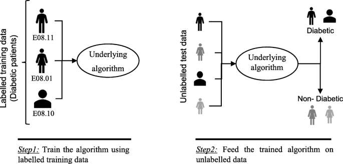
Supervised learning algorithms In supervised learning, the machine is expected to deliver known outcomes. The training data is already supplied with predefined labels or outcomes. The algorithm has to identify matching characteristics or common features among training data that reference predefined labels/outcomes. Post-training, the same features/attributes are compared to label unknown data.
For example, a microcomputer may be supplied with a sensor dataset of temperature, light, and humidity. Then, it may be modeled to predict day or night or estimate the time of the day. In such a case, in contrast to a typical embedded program routine, a machine learning model has better chances to come up with malfunctioning of sensors and sensor variations as the machine could autonomously deal with erroneous input data through a rigorous process of supervised learning. A model is considered to be deployable after a thorough process of test and validation
The two most common learning problems are usually solved by supervised learning are classification and regression. Classification deals with labeling input data with predefined labels. Regression deals with deriving outcomes of unknown input data based on learned correlations between training data and known outcomes. The derived outcome is a numerical value or result.
Some of the common machine learning algorithms that fall under supervised learning include K Nearest Neighbor, Random Forest, Logistic Regression, Decision Trees, and Back Propagation Neural Network.
Unsupervised learning algorithms In unsupervised learning, the machine is expected to deliver unknown outcomes. The machine is exposed to unlabelled raw data samples and it must deduce structures present in the input data. This is usually done mathematically by either extracting similarities or removing redundancies. The outcome of machine learning is not a class/label or a numerical output; instead, the output is delivered by grouping similar data samples or identifying the odd ones.
Some of the common problems solved through unsupervised learning are clustering, association rule mining, and dimensionality reduction. Some of the common machine learning algorithms that fall under unsupervised learning include K-Means Clustering, Apriori Algorithm, KNN, Hierarchal Clustering, Singular Value Decomposition, Anomaly Detection, Principal Component Analysis, Neural Networks, and Independent Component Analysis.
Semi-supervised learning algorithms In semi-supervised learning, the machine is trained with labeled datasets then exposed to unknown data samples for deriving common features/associations among data belonging to the same classes. Alternatively, the machine is first trained on unlabelled data to derive its own classes and then the training is refined by providing labeled datasets. In both cases, the machine has to predict expected outcomes (class or a numerical value) as well as deduce inherent patterns within input data. Semi-supervised learning also deals with the same problems that supervised learning does (i.e. classification and regression) albeit, semi-supervised learning is expected to be finer in its outcomes.
Some of the common machine learning algorithms that fall under semi-supervised learning include Continuity Assumption, Generative Models, Laplacian Regularization, Cluster Assumption, Heuristic Approaches, Low-Density Separation, Discrete Regularization, Label Propagation, and Quadratic Criterion, and Manifold Assumption.
Reinforcement learning algorithms In reinforcement learning, a system called an agent is developed to interact in a specific environment so that its performance for executing certain tasks improves from the interactions. The agent starts from a predefined initial set of policies, rules, or strategies and then is exposed to a specific environment in order to observe the environment and its current state. Based on its perception of the environment, it selects an optimal policy/strategy and performs actions. In response to every action, the agent gets feedback from the environment in the form of a reward or penalty. It uses the penalty/reward to update its policy/strategy and again interacts with the environment to repeat actions.
Some of the common machine learning algorithms that fall under reinforcement learning include Q-Learning (State-Action-Reward-State), SARSA (State-Action-Reward-State-Action), Lambda Q-Learning, Lambda SARSA, Deep Q Network, NAF (Normalized Advantage Functions), DDPG (Deep Determinant Policy Gradient), TD3 (Twin Delayed Deep Deterministic Policy Gradient), PPO (Proximal Policy Optimization), A3C (Asynchronous Advantage Actor-Critic Algorithm), SAC (Soft Actor Critic), and TRPO (Trust Religion Policy Optimization).
Narrow classification The classification of ML algorithms based on learning techniques can be short-listed based on their functions or similarities, giving a list of possible algorithms that can be used for a particular learning problem. The rest of the selection of a specific algorithm for a particular problem depends upon the intrinsic details and workings of the shortlisted algorithms and the developer’s own discretion regarding which algorithm will be best suited for a given problem. Machine learning algorithms can be shortlisted as follows on the basis of functions or similarities.
Bayesian Algorithms These are the algorithms that specifically apply Bayes’ Theorem for solving the supervised learning problems (i.e. classification or regression). Some of the algorithms that fall in this category include Naive Bayes, Averaged One-Dependence Estimators (AODE), Gaussian Naive Bayes, Multinomial Naive Bayes, Bayesian Network (BN), and Bayesian Belief Network (BNN).
Regression Algorithms Regression algorithms are focused on deriving a numerical output based on input data. The machine is trained on data for which the outcomes are already known. Once the training is done, the machine attempts to improve outcomes by redundantly measuring errors in the prediction of the outcomes. Regression is basically a machine learning problem and statistical method, as well as an algorithm. Some of the algorithms that fall in this category include Linear Regression, Stepwise Regression, Logistic Regression, Ordinary Least Squares Regression, Locally Estimated Scatterplot Smoothing (LOSS), and Multivariate Adaptive Regression Splines (MARS).
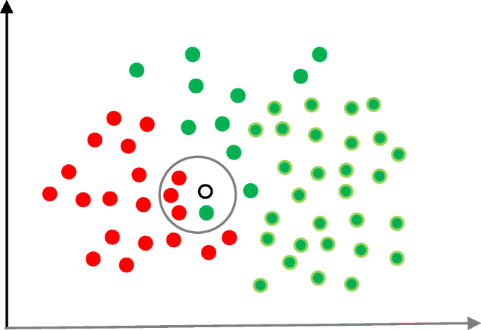
Instance-based algorithms Instance-based algorithms are often used to solve classification problems. A sample training data is stored in a database and, by using various similarity measures, the input data samples are compared with the stored instances. As the stored instances are labeled, those that match a given instance he best are assigned the same class as the input data sample. This is also called memory-based learning. Some of the algorithms that fall in this category include K-Nearest Neighbor (KNN), Self-Organizing Map (SOM), Learning Vector Quantization (LVQ), Support Vector Machines (SVM), and Locally Weighted Learning (LWL).
Regularization algorithms Regularization algorithms are similar to regression algorithms, although they have provisions to penalize models on the basis of their complexity. Such algorithms are excellent in generalizing the outcome. Some of the common algorithms that fall in this category include Least Absolute Shrinkage and Selection Operator (LASSO), Least Angle Regression (LARS), Ridge Regression, and Elastic Net.
Decision tree algorithms In decision tree algorithms, specific and well-defined attributes of input data are matched to eventually derive a decision. These algorithms are extremely fast and highly accurate as the decision are made step-by-step based on well-defined parameters. These algorithms are used for bot classification and regression problems. Some of the common algorithms that fall in this category include Decision Stump, Conditional Decision Trees, Classification and Regression Tree (CART), M5, C4.5, C5.0, Iterative Dichotomiser 3 (ID3), and Chi-Squared Automatic Interaction Detection (CHAID).
Clustering algorithms The clustering algorithms are usually aimed to solve classification problems. These algorithms are, however, tuned to work upon unlabelled data. They focus on extracting inherent patterns of the data samples and group the data samples into distinct classes. Some of the common algorithms that fall in this category include K-Means, K-Medians, Hierarchical clustering, and Expectation Maximization (EM).
Dimensionality reduction algorithms The dimensionality reduction algorithms are similar to clustering algorithms. The difference is that these algorithms do not attempt to classify data under distinct labels. Instead, the algorithms focus on exploring inherent patterns in order to simplify and summarize data points. These algorithms are used for solving both classification and regression problems. Some of the common algorithms that fall in this category include Sammon Mapping, Principal Component Analysis (PCA), Principal Component Regression (PCR), Projection Pursuit, Partial Least Squares Regression (PLSR), Multidimensional Scaling, Linear Discriminant Analysis (LDA), Quadratic Discriminant Analysis (QDA), Mixture Discriminant Analysis (MDA), and Flexible Discriminant Analysis (FDA).
Association rule learning algorithms These algorithms are focused on deducing rules governing relationships between data variables. The most popular association rule learning algorithms are Eclat Algorithm and Apriori Algorithm.
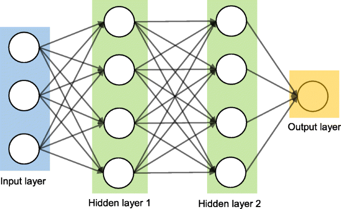
Artificial neural network algorithms These algorithms are based on the use of artificial neural networks (ANN) and are used to solve both classification and regression problems. Artificial neural networks are data structures comprising of multiple layers, which include an input layer, an output layer, and one or several hidden layers. The hidden layers manipulate input data to derive useful representations of the data samples. The representations are adjusted in multiple hidden layers until an appropriate association between input data and output values is established. The fundamental ANN algorithms include Perceptron, Back Propagation, Hopfield Network, Multilayer Perceptrons, Stochastic Gradient Descent, and Radial Basis Function Network. Actually, there are hundreds of such algorithms. ANN are inspired by the functioning of biological neural networks and are similarly structured.
Deep learning algorithms Deep learning algorithms also use artificial neural networks; however, they are different from traditional ANN-based algorithms. The deep learning algorithms are tuned to perform a large volume of simple computations. These algorithms often deal with analog data such as images, videos, text, and sensor values. Some of the popular deep learning algorithms include Convolutional Neural Networks (CNN), Recurrent Neural Networks (RNN), Deep Belief Networks (DBN), Long Short-Term Memory Networks (LSTM), Deep Boltzmann Machine (DBM), and Stacked Auto-Encoders.
Ensemble algorithms In these algorithms, multiple models are independently trained and their outcomes are combined to derive a final outcome. They are very powerful as multiple models are carefully combined to maximize the overall accuracy and performance. Some of the algorithms that fall in this category include Random Forrest, Gradient Boosting Machines (GBM), Weighted Average Blending, Bootstrapped Aggregation or Bagging, Gradient Boosted Regression Trees (GBRT), Stacking, AdaBoost, and Boosting.
Conclusion With hundreds of algorithms available, it can be a daunting task to select one machine learning algorithm for solving a given problem. The selection becomes simpler by first understanding the nature of machine learning or the machine learning technique. The search for an appropriate algorithm can be further refined by listing algorithms for the desired function or task. From there, the applicability, advantages, disadvantages, and available resources must be considered for selecting the right algorithm.
You may also like:
What is TinyML?
What is machine learning?
What are different types of Artificial Intelligence ?
What is Artificial Intelligence, Machine Learning, Deep Learning, and Natural…
Introduction to Robotics
Artificial Intelligence vs. Intelligence Augmentation
Supervised learning is an area of machine learning where the chosen algorithm tries to fit a target using the given input. A set of training data that contains labels is supplied to the algorithm. Based on a massive set of data, the algorithm will learn a rule that it uses to predict the labels for new observations. In other words, supervised learning algorithms are provided with historical data and asked to find the relationship that has the best predictive power.
There are two varieties of supervised learning algorithms: regression and classification algorithms. Regression-based supervised learning methods try to predict outputs based on input variables. Classification-based supervised learning methods identify which category a set of data items belongs to. Classification algorithms are probability-based, meaning the outcome is the category for which the algorithm finds the highest probability that the dataset belongs to it. Regression algorithms, in contrast, estimate the outcome of problems that have an infinite number of solutions (continuous set of possible outcomes).
In the context of finance, supervised learning models represent one of the most-used class of machine learning models. Many algorithms that are widely applied in algorithmic trading rely on supervised learning models because they can be efficiently trained, they are relatively robust to noisy financial data, and they have strong links to the theory of finance.
Regression-based algorithms have been leveraged by academic and industry researchers to develop numerous asset pricing models. These models are used to predict returns over various time periods and to identify significant factors that drive asset returns. There are many other use cases of regression-based supervised learning in portfolio management and derivatives pricing.
Classification-based algorithms, on the other hand, have been leveraged across many areas within finance that require predicting a categorical response. These include fraud detection, default prediction, credit scoring, directional forecast of asset price movement, and Buy/Sell recommendations. There are many other use cases of classification-based supervised learning in portfolio management and algorithmic trading.
Many use cases of regression-based and classification-based supervised machine learning are presented in Chapters 5 and 6.
Python and its libraries provide methods and ways to implement these supervised learning models in few lines of code. Some of these libraries were covered in Chapter 2. With easy-to-use machine learning libraries like Scikit-learn and Keras, it is straightforward to fit different machine learning models on a given predictive modeling dataset.
In this chapter, we present a high-level overview of supervised learning models. For a thorough coverage of the topics, the reader is referred to Hands-On Machine Learning with Scikit-Learn, Keras, and TensorFlow, 2nd Edition, by Aurélien Géron (O’Reilly).
The following topics are covered in this chapter:
Basic concepts of supervised learning models (both regression and classification).
How to implement different supervised learning models in Python.
How to tune the models and identify the optimal parameters of the models using grid search.
Overfitting versus underfitting and bias versus variance.
Strengths and weaknesses of several supervised learning models.
How to use ensemble models, ANN, and deep learning models for both regression and classification.
How to select a model on the basis of several factors, including model performance.
Evaluation metrics for classification and regression models.
How to perform cross validation.
Supervised Learning Models: An Overview
Classification predictive modeling problems are different from regression predictive modeling problems, as classification is the task of predicting a discrete class label and regression is the task of predicting a continuous quantity. However, both share the same concept of utilizing known variables to make predictions, and there is a significant overlap between the two models. Hence, the models for classification and regression are presented together in this chapter. Figure 4-1 summarizes the list of the models commonly used for classification and regression.
Some models can be used for both classification and regression with small modifications. These are K-nearest neighbors, decision trees, support vector, ensemble bagging/boosting methods, and ANNs (including deep neural networks), as shown in Figure 4-1. However, some models, such as linear regression and logistic regression, cannot (or cannot easily) be used for both problem types.
This section contains the following details about the models:
Theory of the models.
Implementation in Scikit-learn or Keras.
Grid search for different models.
Pros and cons of the models.
Note
In finance, a key focus is on models that extract signals from previously observed data in order to predict future values for the same time series. This family of time series models predicts continuous output and is more aligned with the supervised regression models. Time series models are covered separately in the supervised regression chapter (Chapter 5).
Linear Regression (Ordinary Least Squares)
Linear regression (Ordinary Least Squares Regression or OLS Regression) is perhaps one of the most well-known and best-understood algorithms in statistics and machine learning. Linear regression is a linear model, e.g., a model that assumes a linear relationship between the input variables (x) and the single output variable (y). The goal of linear regression is to train a linear model to predict a new y given a previously unseen x with as little error as possible.
Our model will be a function that predicts y given �1,�2…��:�=�0+�1�1+…+����
where, �0 is called intercept and �1…�� are the coefficient of the regression.
In the following section, we cover the training of a linear regression model and grid search of the model. However, the overall concepts and related approaches are applicable to all other supervised learning models.
Training a model
As we mentioned in Chapter 3, training a model basically means retrieving the model parameters by minimizing the cost (loss) function. The two steps for training a linear regression model are:Define a cost function (or loss function)
Measures how inaccurate the model’s predictions are. The sum of squared residuals (RSS) as defined in Equation 4-1 measures the squared sum of the difference between the actual and predicted value and is the cost function for linear regression.
Equation 4-1. Sum of squared residuals
���=∑�=1���–�0–∑�=1������2
In this equation, �0 is the intercept; �� represents the coefficient; �1,..,�� are the coefficients of the regression; and ��� represents the ��ℎ observation and ��ℎ variable.Find the parameters that minimize loss
For example, make our model as accurate as possible. Graphically, in two dimensions, this results in a line of best fit as shown in Figure 4-2. In higher dimensions, we would have higher-dimensional hyperplanes. Mathematically, we look at the difference between each real data point (y) and our model’s prediction (ŷ). Square these differences to avoid negative numbers and penalize larger differences, and then add them up and take the average. This is a measure of how well our data fits the line.
Grid search
The overall idea of the grid search is to create a grid of all possible hyperparameter combinations and train the model using each one of them. Hyperparameters are the external characteristic of the model, can be considered the model’s settings, and are not estimated based on data-like model parameters. These hyperparameters are tuned during grid search to achieve better model performance.
Due to its exhaustive search, a grid search is guaranteed to find the optimal parameter within the grid. The drawback is that the size of the grid grows exponentially with the addition of more parameters or more considered values.
The GridSearchCV class in the model_selection module of the sklearn package facilitates the systematic evaluation of all combinations of the hyperparameter values that we would like to test.
The first step is to create a model object. We then define a dictionary where the keywords name the hyperparameters and the values list the parameter settings to be tested. For linear regression, the hyperparameter is fit_intercept, which is a boolean variable that determines whether or not to calculate the intercept for this model. If set to False, no intercept will be used in calculations:
The second step is to instantiate the GridSearchCV object and provide the estimator object and parameter grid, as well as a scoring method and cross validation choice, to the initialization method. Cross validation is a resampling procedure used to evaluate machine learning models, and scoring parameter is the evaluation metrics of the model:1
With all settings in place, we can fit GridSearchCV:
In terms of advantages, linear regression is easy to understand and interpret. However, it may not work well when there is a nonlinear relationship between predicted and predictor variables. Linear regression is prone to overfitting (which we will discuss in the next section) and when a large number of features are present, it may not handle irrelevant features well. Linear regression also requires the data to follow certain assumptions, such as the absence of multicollinearity. If the assumptions fail, then we cannot trust the results obtained.
Regularized Regression
When a linear regression model contains many independent variables, their coefficients will be poorly determined, and the model will have a tendency to fit extremely well to the training data (data used to build the model) but fit poorly to testing data (data used to test how good the model is). This is known as overfitting or high variance.
One popular technique to control overfitting is regularization, which involves the addition of a penalty term to the error or loss function to discourage the coefficients from reaching large values. Regularization, in simple terms, is a penalty mechanism that applies shrinkage to model parameters (driving them closer to zero) in order to build a model with higher prediction accuracy and interpretation. Regularized regression has two advantages over linear regression:Prediction accuracy
The performance of the model working better on the testing data suggests that the model is trying to generalize from training data. A model with too many parameters might try to fit noise specific to the training data. By shrinking or setting some coefficients to zero, we trade off the ability to fit complex models (higher bias) for a more generalizable model (lower variance).Interpretation
A large number of predictors may complicate the interpretation or communication of the big picture of the results. It may be preferable to sacrifice some detail to limit the model to a smaller subset of parameters with the strongest effects.
The common ways to regularize a linear regression model are as follows:L1 regularization or Lasso regression
Lasso regression performs L1 regularization by adding a factor of the sum of the absolute value of coefficients in the cost function (RSS) for linear regression, as mentioned in Equation 4-1. The equation for lasso regularization can be represented as follows:
������������=���+�*∑�=1���
L1 regularization can lead to zero coefficients (i.e., some of the features are completely neglected for the evaluation of output). The larger the value of �, the more features are shrunk to zero. This can eliminate some features entirely and give us a subset of predictors, reducing model complexity. So Lasso regression not only helps in reducing overfitting, but also can help in feature selection. Predictors not shrunk toward zero signify that they are important, and thus L1 regularization allows for feature selection (sparse selection). The regularization parameter (�) can be controlled, and a lambda value of zero produces the basic linear regression equation.
A lasso regression model can be constructed using the Lasso class of the sklearn package of Python, as shown in the code snippet that follows:
Ridge regression performs L2 regularization by adding a factor of the sum of the square of coefficients in the cost function (RSS) for linear regression, as mentioned in Equation 4-1. The equation for ridge regularization can be represented as follows:
������������=���+�*∑�=1���2
Ridge regression puts constraint on the coefficients. The penalty term (�) regularizes the coefficients such that if the coefficients take large values, the optimization function is penalized. So ridge regression shrinks the coefficients and helps to reduce the model complexity. Shrinking the coefficients leads to a lower variance and a lower error value. Therefore, ridge regression decreases the complexity of a model but does not reduce the number of variables; it just shrinks their effect. When � is closer to zero, the cost function becomes similar to the linear regression cost function. So the lower the constraint (low �) on the features, the more the model will resemble the linear regression model.
A ridge regression model can be constructed using the Ridge class of the sklearn package of Python, as shown in the code snippet that follows:
Elastic nets add regularization terms to the model, which are a combination of both L1 and L2 regularization, as shown in the following equation:
������������=���+�*(1–�)/2*∑�=1���2+�*∑�=1���
In addition to setting and choosing a � value, an elastic net also allows us to tune the alpha parameter, where � = 0 corresponds to ridge and � = 1 to lasso. Therefore, we can choose an � value between 0 and 1 to optimize the elastic net. Effectively, this will shrink some coefficients and set some to 0 for sparse selection.
An elastic net regression model can be constructed using the ElasticNet class of the sklearn package of Python, as shown in the following code snippet:
For all the regularized regression, � is the key parameter to tune during grid search in Python. In an elastic net, � can be an additional parameter to tune.
Logistic Regression
Logistic regression is one of the most widely used algorithms for classification. The logistic regression model arises from the desire to model the probabilities of the output classes given a function that is linear in x, at the same time ensuring that output probabilities sum up to one and remain between zero and one as we would expect from probabilities.
If we train a linear regression model on several examples where Y = 0 or 1, we might end up predicting some probabilities that are less than zero or greater than one, which doesn’t make sense. Instead, we use a logistic regression model (or logit model), which is a modification of linear regression that makes sure to output a probability between zero and one by applying the sigmoid function.2
Equation 4-2 shows the equation for a logistic regression model. Similar to linear regression, input values (x) are combined linearly using weights or coefficient values to predict an output value (y). The output coming from Equation 4-2 is a probability that is transformed into a binary value (0 or 1) to get the model prediction.
Equation 4-2. Logistic regression equation
�=exp(�0+�1�1+….+���1)1+exp(�0+�1�1+….+���1)
Where y is the predicted output, �0 is the bias or intercept term and B1 is the coefficient for the single input value (x). Each column in the input data has an associated � coefficient (a constant real value) that must be learned from the training data.
In logistic regression, the cost function is basically a measure of how often we predicted one when the true answer was zero, or vice versa. Training the logistic regression coefficients is done using techniques such as maximum likelihood estimation (MLE) to predict values close to 1 for the default class and close to 0 for the other class.3
A logistic regression model can be constructed using the LogisticRegression class of the sklearn package of Python, as shown in the following code snippet:
Similar to linear regression, logistic regression can have regularization, which can be L1, L2, or elasticnet. The values in the sklearn library are [l1, l2, elasticnet].Regularization strength (C in sklearn)
This parameter controls the regularization strength. Good values of the penalty parameters can be [100, 10, 1.0, 0.1, 0.01].
Advantages and disadvantages
In terms of the advantages, the logistic regression model is easy to implement, has good interpretability, and performs very well on linearly separable classes. The output of the model is a probability, which provides more insight and can be used for ranking. The model has small number of hyperparameters. Although there may be risk of overfitting, this may be addressed using L1/L2 regularization, similar to the way we addressed overfitting for the linear regression models.
In terms of disadvantages, the model may overfit when provided with large numbers of features. Logistic regression can only learn linear functions and is less suitable to complex relationships between features and the target variable. Also, it may not handle irrelevant features well, especially if the features are strongly correlated.
Support Vector Machine
The objective of the support vector machine (SVM) algorithm is to maximize the margin (shown as shaded area in Figure 4-3), which is defined as the distance between the separating hyperplane (or decision boundary) and the training samples that are closest to this hyperplane, the so-called support vectors. The margin is calculated as the perpendicular distance from the line to only the closest points, as shown in Figure 4-3. Hence, SVM calculates a maximum-margin boundary that leads to a homogeneous partition of all data points.
In practice, the data is messy and cannot be separated perfectly with a hyperplane. The constraint of maximizing the margin of the line that separates the classes must be relaxed. This change allows some points in the training data to violate the separating line. An additional set of coefficients is introduced that give the margin wiggle room in each dimension. A tuning parameter is introduced, simply called C, that defines the magnitude of the wiggle allowed across all dimensions. The larger the value of C, the more violations of the hyperplane are permitted.
In some cases, it is not possible to find a hyperplane or a linear decision boundary, and kernels are used. A kernel is just a transformation of the input data that allows the SVM algorithm to treat/process the data more easily. Using kernels, the original data is projected into a higher dimension to classify the data better.
SVM is used for both classification and regression. We achieve this by converting the original optimization problem into a dual problem. For regression, the trick is to reverse the objective. Instead of trying to fit the largest possible street between two classes while limiting margin violations, SVM regression tries to fit as many instances as possible on the street (shaded area in Figure 4-3) while limiting margin violations. The width of the street is controlled by a hyperparameter.
The SVM regression and classification models can be constructed using the sklearn package of Python, as shown in the following code snippets:
Regression
fromsklearn.svmimportSVRmodel=SVR()model.fit(X,Y)
Classification
fromsklearn.svmimportSVCmodel=SVC()model.fit(X,Y)
Hyperparameters
The following key parameters are present in the sklearn implementation of SVM and can be tweaked while performing the grid search:Kernels (kernel in sklearn)
The choice of kernel controls the manner in which the input variables will be projected. There are many kernels to choose from, but linear and RBF are the most common.Penalty (C in sklearn)
The penalty parameter tells the SVM optimization how much you want to avoid misclassifying each training example. For large values of the penalty parameter, the optimization will choose a smaller-margin hyperplane. Good values might be a log scale from 10 to 1,000.
Advantages and disadvantages
In terms of advantages, SVM is fairly robust against overfitting, especially in higher dimensional space. It handles the nonlinear relationships quite well, with many kernels to choose from. Also, there is no distributional requirement for the data.
In terms of disadvantages, SVM can be inefficient to train and memory-intensive to run and tune. It doesn’t perform well with large datasets. It requires the feature scaling of the data. There are also many hyperparameters, and their meanings are often not intuitive.
K-Nearest Neighbors
K-nearest neighbors (KNN) is considered a “lazy learner,” as there is no learning required in the model. For a new data point, predictions are made by searching through the entire training set for the K most similar instances (the neighbors) and summarizing the output variable for those K instances.
To determine which of the K instances in the training dataset are most similar to a new input, a distance measure is used. The most popular distance measure is Euclidean distance, which is calculated as the square root of the sum of the squared differences between a point a and a point b across all input attributes i, and which is represented as �(�,�)=∑�=1�(��–��)2. Euclidean distance is a good distance measure to use if the input variables are similar in type.
Another distance metric is Manhattan distance, in which the distance between point a and point b is represented as �(�,�)=∑�=1�|��–��|. Manhattan distance is a good measure to use if the input variables are not similar in type.
The steps of KNN can be summarized as follows:
Choose the number of K and a distance metric.
Find the K-nearest neighbors of the sample that we want to classify.
Assign the class label by majority vote.
KNN regression and classification models can be constructed using the sklearn package of Python, as shown in the following code:
The following key parameters are present in the sklearn implementation of KNN and can be tweaked while performing the grid search:Number of neighbors (n_neighbors in sklearn)
The most important hyperparameter for KNN is the number of neighbors (n_neighbors). Good values are between 1 and 20.Distance metric (metric in sklearn)
It may also be interesting to test different distance metrics for choosing the composition of the neighborhood. Good values are euclidean and manhattan.
Advantages and disadvantages
In terms of advantages, no training is involved and hence there is no learning phase. Since the algorithm requires no training before making predictions, new data can be added seamlessly without impacting the accuracy of the algorithm. It is intuitive and easy to understand. The model naturally handles multiclass classification and can learn complex decision boundaries. KNN is effective if the training data is large. It is also robust to noisy data, and there is no need to filter the outliers.
In terms of the disadvantages, the distance metric to choose is not obvious and difficult to justify in many cases. KNN performs poorly on high dimensional datasets. It is expensive and slow to predict new instances because the distance to all neighbors must be recalculated. KNN is sensitive to noise in the dataset. We need to manually input missing values and remove outliers. Also, feature scaling (standardization and normalization) is required before applying the KNN algorithm to any dataset; otherwise, KNN may generate wrong predictions.
Linear Discriminant Analysis
The objective of the linear discriminant analysis (LDA) algorithm is to project the data onto a lower-dimensional space in a way that the class separability is maximized and the variance within a class is minimized.4
During the training of the LDA model, the statistical properties (i.e., mean and covariance matrix) of each class are computed. The statistical properties are estimated on the basis of the following assumptions about the data:
Data is normally distributed, so that each variable is shaped like a bell curve when plotted.
Each attribute has the same variance, and the values of each variable vary around the mean by the same amount on average.
To make a prediction, LDA estimates the probability that a new set of inputs belongs to every class. The output class is the one that has the highest probability.
Implementation in Python and hyperparameters
The LDA classification model can be constructed using the sklearn package of Python, as shown in the following code snippet:
The key hyperparameter for the LDA model is number of components for dimensionality reduction, which is represented by n_components in sklearn.
Advantages and disadvantages
In terms of advantages, LDA is a relatively simple model with fast implementation and is easy to implement. In terms of disadvantages, it requires feature scaling and involves complex matrix operations.
Classification and Regression Trees
In the most general terms, the purpose of an analysis via tree-building algorithms is to determine a set of if–then logical (split) conditions that permit accurate prediction or classification of cases. Classification and regression trees (or CART or decision tree classifiers) are attractive models if we care about interpretability. We can think of this model as breaking down our data and making a decision based on asking a series of questions. This algorithm is the foundation of ensemble methods such as random forest and gradient boosting method.
Representation
The model can be represented by a binary tree (or decision tree), where each node is an input variable x with a split point and each leaf contains an output variable y for prediction.
Figure 4-4 shows an example of a simple classification tree to predict whether a person is a male or a female based on two inputs of height (in centimeters) and weight (in kilograms).
Learning a CART model
Creating a binary tree is actually a process of dividing up the input space. A greedy approach called recursive binary splitting is used to divide the space. This is a numerical procedure in which all the values are lined up and different split points are tried and tested using a cost (loss) function. The split with the best cost (lowest cost, because we minimize cost) is selected. All input variables and all possible split points are evaluated and chosen in a greedy manner (e.g., the very best split point is chosen each time).
For regression predictive modeling problems, the cost function that is minimized to choose split points is the sum of squared errors across all training samples that fall within the rectangle:∑�=1�(��–�����������)2
where �� is the output for the training sample and prediction is the predicted output for the rectangle. For classification, the Gini cost function is used; it provides an indication of how pure the leaf nodes are (i.e., how mixed the training data assigned to each node is) and is defined as:�=∑�=1���*(1–��)
where G is the Gini cost over all classes and �� is the number of training instances with class k in the rectangle of interest. A node that has all classes of the same type (perfect class purity) will have G = 0, while a node that has a 50–50 split of classes for a binary classification problem (worst purity) will have G = 0.5.
Stopping criterion
The recursive binary splitting procedure described in the preceding section needs to know when to stop splitting as it works its way down the tree with the training data. The most common stopping procedure is to use a minimum count on the number of training instances assigned to each leaf node. If the count is less than some minimum, then the split is not accepted and the node is taken as a final leaf node.
Pruning the tree
The stopping criterion is important as it strongly influences the performance of the tree. Pruning can be used after learning the tree to further lift performance. The complexity of a decision tree is defined as the number of splits in the tree. Simpler trees are preferred as they are faster to run and easy to understand, consume less memory during processing and storage, and are less likely to overfit the data. The fastest and simplest pruning method is to work through each leaf node in the tree and evaluate the effect of removing it using a test set. A leaf node is removed only if doing so results in a drop in the overall cost function on the entire test set. The removal of nodes can be stopped when no further improvements can be made.
Implementation in Python
CART regression and classification models can be constructed using the sklearn package of Python, as shown in the following code snippet:
CART has many hyperparameters. However, the key hyperparameter is the maximum depth of the tree model, which is the number of components for dimensionality reduction, and which is represented by max_depth in the sklearn package. Good values can range from 2 to 30 depending on the number of features in the data.
Advantages and disadvantages
In terms of advantages, CART is easy to interpret and can adapt to learn complex relationships. It requires little data preparation, and data typically does not need to be scaled. Feature importance is built in due to the way decision nodes are built. It performs well on large datasets. It works for both regression and classification problems.
In terms of disadvantages, CART is prone to overfitting unless pruning is used. It can be very nonrobust, meaning that small changes in the training dataset can lead to quite major differences in the hypothesis function that gets learned. CART generally has worse performance than ensemble models, which are covered next.
Ensemble Models
The goal of ensemble models is to combine different classifiers into a meta-classifier that has better generalization performance than each individual classifier alone. For example, assuming that we collected predictions from 10 experts, ensemble methods would allow us to strategically combine their predictions to come up with a prediction that is more accurate and robust than the experts’ individual predictions.
The two most popular ensemble methods are bagging and boosting. Bagging (or bootstrap aggregation) is an ensemble technique of training several individual models in a parallel way. Each model is trained by a random subset of the data. Boosting, on the other hand, is an ensemble technique of training several individual models in a sequential way. This is done by building a model from the training data and then creating a second model that attempts to correct the errors of the first model. Models are added until the training set is predicted perfectly or a maximum number of models is added. Each individual model learns from mistakes made by the previous model. Just like the decision trees themselves, bagging and boosting can be used for classification and regression problems.
By combining individual models, the ensemble model tends to be more flexible (less bias) and less data-sensitive (less variance).5 Ensemble methods combine multiple, simpler algorithms to obtain better performance.
In this section we will cover random forest, AdaBoost, the gradient boosting method, and extra trees, along with their implementation using sklearn package.
Random forest
Random forest is a tweaked version of bagged decision trees. In order to understand a random forest algorithm, let us first understand the bagging algorithm. Assuming we have a dataset of one thousand instances, the steps of bagging are:
Create many (e.g., one hundred) random subsamples of our dataset.
Train a CART model on each sample.
Given a new dataset, calculate the average prediction from each model and aggregate the prediction by each tree to assign the final label by majority vote.
A problem with decision trees like CART is that they are greedy. They choose the variable to split by using a greedy algorithm that minimizes error. Even after bagging, the decision trees can have a lot of structural similarities and result in high correlation in their predictions. Combining predictions from multiple models in ensembles works better if the predictions from the submodels are uncorrelated, or at best are weakly correlated. Random forest changes the learning algorithm in such a way that the resulting predictions from all of the subtrees have less correlation.
In CART, when selecting a split point, the learning algorithm is allowed to look through all variables and all variable values in order to select the most optimal split point. The random forest algorithm changes this procedure such that each subtree can access only a random sample of features when selecting the split points. The number of features that can be searched at each split point (m) must be specified as a parameter to the algorithm.
As the bagged decision trees are constructed, we can calculate how much the error function drops for a variable at each split point. In regression problems, this may be the drop in sum squared error, and in classification, this might be the Gini cost. The bagged method can provide feature importance by calculating and averaging the error function drop for individual variables.
Implementation in Python
Random forest regression and classification models can be constructed using the sklearn package of Python, as shown in the following code:
Some of the main hyperparameters that are present in the sklearn implementation of random forest and that can be tweaked while performing the grid search are:Maximum number of features (max_features in sklearn)
This is the most important parameter. It is the number of random features to sample at each split point. You could try a range of integer values, such as 1 to 20, or 1 to half the number of input features.Number of estimators (n_estimators in sklearn)
This parameter represents the number of trees. Ideally, this should be increased until no further improvement is seen in the model. Good values might be a log scale from 10 to 1,000.
Advantages and disadvantages
The random forest algorithm (or model) has gained huge popularity in ML applications during the last decade due to its good performance, scalability, and ease of use. It is flexible and naturally assigns feature importance scores, so it can handle redundant feature columns. It scales to large datasets and is generally robust to overfitting. The algorithm doesn’t need the data to be scaled and can model a nonlinear relationship.
In terms of disadvantages, random forest can feel like a black box approach, as we have very little control over what the model does, and the results may be difficult to interpret. Although random forest does a good job at classification, it may not be good for regression problems, as it does not give a precise continuous nature prediction. In the case of regression, it doesn’t predict beyond the range in the training data and may overfit datasets that are particularly noisy.
Extra trees
Extra trees, otherwise known as extremely randomized trees, is a variant of a random forest; it builds multiple trees and splits nodes using random subsets of features similar to random forest. However, unlike random forest, where observations are drawn with replacement, the observations are drawn without replacement in extra trees. So there is no repetition of observations.
Additionally, random forest selects the best split to convert the parent into the two most homogeneous child nodes.6 However, extra trees selects a random split to divide the parent node into two random child nodes. In extra trees, randomness doesn’t come from bootstrapping the data; it comes from the random splits of all observations.
In real-world cases, performance is comparable to an ordinary random forest, sometimes a bit better. The advantages and disadvantages of extra trees are similar to those of random forest.
Implementation in Python
Extra trees regression and classification models can be constructed using the sklearn package of Python, as shown in the following code snippet. The hyperparameters of extra trees are similar to random forest, as shown in the previous section:
Adaptive Boosting or AdaBoost is a boosting technique in which the basic idea is to try predictors sequentially, and each subsequent model attempts to fix the errors of its predecessor. At each iteration, the AdaBoost algorithm changes the sample distribution by modifying the weights attached to each of the instances. It increases the weights of the wrongly predicted instances and decreases the ones of the correctly predicted instances.
The steps of the AdaBoost algorithm are:
Initially, all observations are given equal weights.
A model is built on a subset of data, and using this model, predictions are made on the whole dataset. Errors are calculated by comparing the predictions and actual values.
While creating the next model, higher weights are given to the data points that were predicted incorrectly. Weights can be determined using the error value. For instance, the higher the error, the more weight is assigned to the observation.
This process is repeated until the error function does not change, or until the maximum limit of the number of estimators is reached.
Implementation in Python
AdaBoost regression and classification models can be constructed using the sklearn package of Python, as shown in the following code snippet:
Some of the main hyperparameters that are present in the sklearn implementation of AdaBoost and that can be tweaked while performing the grid search are as follows:Learning rate (learning_rate in sklearn)
Learning rate shrinks the contribution of each classifier/regressor. It can be considered on a log scale. The sample values for grid search can be 0.001, 0.01, and 0.1.Number of estimators (n_estimators in sklearn)
This parameter represents the number of trees. Ideally, this should be increased until no further improvement is seen in the model. Good values might be a log scale from 10 to 1,000.
Advantages and disadvantages
In terms of advantages, AdaBoost has a high degree of precision. AdaBoost can achieve similar results to other models with much less tweaking of parameters or settings. The algorithm doesn’t need the data to be scaled and can model a nonlinear relationship.
In terms of disadvantages, the training of AdaBoost is time consuming. AdaBoost can be sensitive to noisy data and outliers, and data imbalance leads to a decrease in classification accuracy
Gradient boosting method
Gradient boosting method (GBM) is another boosting technique similar to AdaBoost, where the general idea is to try predictors sequentially. Gradient boosting works by sequentially adding the previous underfitted predictions to the ensemble, ensuring the errors made previously are corrected.
The following are the steps of the gradient boosting algorithm:
A model (which can be referred to as the first weak learner) is built on a subset of data. Using this model, predictions are made on the whole dataset.
Errors are calculated by comparing the predictions and actual values, and the loss is calculated using the loss function.
A new model is created using the errors of the previous step as the target variable. The objective is to find the best split in the data to minimize the error. The predictions made by this new model are combined with the predictions of the previous. New errors are calculated using this predicted value and actual value.
This process is repeated until the error function does not change or until the maximum limit of the number of estimators is reached.
Contrary to AdaBoost, which tweaks the instance weights at every interaction, this method tries to fit the new predictor to the residual errors made by the previous predictor.
Implementation in Python and hyperparameters
Gradient boosting method regression and classification models can be constructed using the sklearn package of Python, as shown in the following code snippet. The hyperparameters of gradient boosting method are similar to AdaBoost, as shown in the previous section:
In terms of advantages, gradient boosting method is robust to missing data, highly correlated features, and irrelevant features in the same way as random forest. It naturally assigns feature importance scores, with slightly better performance than random forest. The algorithm doesn’t need the data to be scaled and can model a nonlinear relationship.
In terms of disadvantages, it may be more prone to overfitting than random forest, as the main purpose of the boosting approach is to reduce bias and not variance. It has many hyperparameters to tune, so model development may not be as fast. Also, feature importance may not be robust to variation in the training dataset.
ANN-Based Models
In Chapter 3 we covered the basics of ANNs, along with the architecture of ANNs and their training and implementation in Python. The details provided in that chapter are applicable across all areas of machine learning, including supervised learning. However, there are a few additional details from the supervised learning perspective, which we will cover in this section.
Neural networks are reducible to a classification or regression model with the activation function of the node in the output layer. In the case of a regression problem, the output node has linear activation function (or no activation function). A linear function produces a continuous output ranging from -inf to +inf. Hence, the output layer will be the linear function of the nodes in the layer before the output layer, and it will be a regression-based model.
In the case of a classification problem, the output node has a sigmoid or softmax activation function. A sigmoid or softmax function produces an output ranging from zero to one to represent the probability of target value. Softmax function can also be used for multiple groups for classification.
ANN using sklearn
ANN regression and classification models can be constructed using the sklearn package of Python, as shown in the following code snippet:
As we saw in Chapter 3, ANN has many hyperparameters. Some of the hyperparameters that are present in the sklearn implementation of ANN and can be tweaked while performing the grid search are:Hidden Layers (hidden_layer_sizes in sklearn)
It represents the number of layers and nodes in the ANN architecture. In sklearn implementation of ANN, the ith element represents the number of neurons in the ith hidden layer. A sample value for grid search in the sklearn implementation can be [(20,), (50,), (20, 20), (20, 30, 20)].Activation Function (activation in sklearn)
It represents the activation function of a hidden layer. Some of the activation functions defined in Chapter 3, such as sigmoid, relu, or tanh, can be used.
Deep neural network
ANNs with more than a single hidden layer are often called deep networks. We prefer using the library Keras to implement such networks, given the flexibility of the library. The detailed implementation of a deep neural network in Keras was shown in Chapter 3. Similar to MLPClassifier and MLPRegressor in sklearn for classification and regression, Keras has modules called KerasClassifier and KerasRegressor that can be used for creating classification and regression models with deep network.
A popular problem in finance is time series prediction, which is predicting the next value of a time series based on a historical overview. Some of the deep neural networks, such as recurrent neural network (RNN), can be directly used for time series prediction. The details of this approach are provided in Chapter 5.
Advantages and disadvantages
The main advantage of an ANN is that it captures the nonlinear relationship between the variables quite well. ANN can more easily learn rich representations and is good with a large number of input features with a large dataset. ANN is flexible in how it can be used. This is evident from its use across a wide variety of areas in machine learning and AI, including reinforcement learning and NLP, as discussed in Chapter 3.
The main disadvantage of ANN is the interpretability of the model, which is a drawback that often cannot be ignored and is sometimes the determining factor when choosing a model. ANN is not good with small datasets and requires a lot of tweaking and guesswork. Choosing the right topology/algorithms to solve a problem is difficult. Also, ANN is computationally expensive and can take a lot of time to train.
Using ANNs for supervised learning in finance
If a simple model such as linear or logistic regression perfectly fits your problem, don’t bother with ANN. However, if you are modeling a complex dataset and feel a need for better prediction power, give ANN a try. ANN is one of the most flexible models in adapting itself to the shape of the data, and using it for supervised learning problems can be an interesting and valuable exercise.
Model Performance
In the previous section, we discussed grid search as a way to find the right hyperparameter to achieve better performance. In this section, we will expand on that process by discussing the key components of evaluating the model performance, which are overfitting, cross validation, and evaluation metrics.
Overfitting and Underfitting
A common problem in machine learning is overfitting, which is defined by learning a function that perfectly explains the training data that the model learned from but doesn’t generalize well to unseen test data. Overfitting happens when a model overlearns from the training data to the point that it starts picking up idiosyncrasies that aren’t representative of patterns in the real world. This becomes especially problematic as we make our models increasingly more complex. Underfitting is a related issue in which the model is not complex enough to capture the underlying trend in the data. Figure 4-5 illustrates overfitting and underfitting. The left-hand panel of Figure 4-5 shows a linear regression model; a straight line clearly underfits the true function. The middle panel shows that a high degree polynomial approximates the true relationship reasonably well. On the other hand, a polynomial of a very high degree fits the small sample almost perfectly, and performs best on the training data, but this doesn’t generalize, and it would do a horrible job at explaining a new data point.
The concepts of overfitting and underfitting are closely linked to bias-variance trade-off. Bias refers to the error due to overly simplistic assumptions or faulty assumptions in the learning algorithm. Bias results in underfitting of the data, as shown in the left-hand panel of Figure 4-5. A high bias means our learning algorithm is missing important trends among the features. Variance refers to the error due to an overly complex model that tries to fit the training data as closely as possible. In high variance cases, the model’s predicted values are extremely close to the actual values from the training set. High variance gives rise to overfitting, as shown in the right-hand panel of Figure 4-5. Ultimately, in order to have a good model, we need low bias and low variance.
There can be two ways to combat overfitting:Using more training data
The more training data we have, the harder it is to overfit the data by learning too much from any single training example.Using regularization
Adding a penalty in the loss function for building a model that assigns too much explanatory power to any one feature, or allows too many features to be taken into account.
The concept of overfitting and the ways to combat it are applicable across all the supervised learning models. For example, regularized regressions address overfitting in linear regression, as discussed earlier in this chapter.
Cross Validation
One of the challenges of machine learning is training models that are able to generalize well to unseen data (overfitting versus underfitting or a bias-variance trade-off). The main idea behind cross validation is to split the data one time or several times so that each split is used once as a validation set and the remainder is used as a training set: part of the data (the training sample) is used to train the algorithm, and the remaining part (the validation sample) is used for estimating the risk of the algorithm. Cross validation allows us to obtain reliable estimates of the model’s generalization error. It is easiest to understand it with an example. When doing k-fold cross validation, we randomly split the training data into k folds. Then we train the model using k-1 folds and evaluate the performance on the kth fold. We repeat this process k times and average the resulting scores.
Figure 4-6 shows an example of cross validation, where the data is split into five sets and in each round one of the sets is used for validation.
A potential drawback of cross validation is the computational cost, especially when paired with a grid search for hyperparameter tuning. Cross validation can be performed in a couple of lines using the sklearn package; we will perform cross validation in the supervised learning case studies.
In the next section, we cover the evaluation metrics for the supervised learning models that are used to measure and compare the models’ performance.
Evaluation Metrics
The metrics used to evaluate the machine learning algorithms are very important. The choice of metrics to use influences how the performance of machine learning algorithms is measured and compared. The metrics influence both how you weight the importance of different characteristics in the results and your ultimate choice of algorithm.
The main evaluation metrics for regression and classification are illustrated in Figure 4-7.
Let us first look at the evaluation metrics for supervised regression.
Mean absolute error
The mean absolute error (MAE) is the sum of the absolute differences between predictions and actual values. The MAE is a linear score, which means that all the individual differences are weighted equally in the average. It gives an idea of how wrong the predictions were. The measure gives an idea of the magnitude of the error, but no idea of the direction (e.g., over- or underpredicting).
Mean squared error
The mean squared error (MSE) represents the sample standard deviation of the differences between predicted values and observed values (called residuals). This is much like the mean absolute error in that it provides a gross idea of the magnitude of the error. Taking the square root of the mean squared error converts the units back to the original units of the output variable and can be meaningful for description and presentation. This is called the root mean squared error (RMSE).
R² metric
The R² metric provides an indication of the “goodness of fit” of the predictions to actual value. In statistical literature this measure is called the coefficient of determination. This is a value between zero and one, for no-fit and perfect fit, respectively.
Adjusted R² metric
Just like R², adjusted R² also shows how well terms fit a curve or line but adjusts for the number of terms in a model. It is given in the following formula:����2=1–(1–�2)(�–1))�–�–1
where n is the total number of observations and k is the number of predictors. Adjusted R² will always be less than or equal to R².
Selecting an evaluation metric for supervised regression
In terms of a preference among these evaluation metrics, if the main goal is predictive accuracy, then RMSE is best. It is computationally simple and is easily differentiable. The loss is symmetric, but larger errors weigh more in the calculation. The MAEs are symmetric but do not weigh larger errors more. R² and adjusted R² are often used for explanatory purposes by indicating how well the selected independent variable(s) explains the variability in the dependent variable(s).
Let us first look at the evaluation metrics for supervised classification.
Classification
For simplicity, we will mostly discuss things in terms of a binary classification problem (i.e., only two outcomes, such as true or false); some common terms are:True positives (TP)
Predicted positive and are actually positive.False positives (FP)
Predicted positive and are actually negative.True negatives (TN)
Predicted negative and are actually negative.False negatives (FN)
Predicted negative and are actually positive.
The difference between three commonly used evaluation metrics for classification, accuracy, precision, and recall, is illustrated in Figure 4-8.
Accuracy
As shown in Figure 4-8, accuracy is the number of correct predictions made as a ratio of all predictions made. This is the most common evaluation metric for classification problems and is also the most misused. It is most suitable when there are an equal number of observations in each class (which is rarely the case) and when all predictions and the related prediction errors are equally important, which is often not the case.
Precision
Precision is the percentage of positive instances out of the total predicted positive instances. Here, the denominator is the model prediction done as positive from the whole given dataset. Precision is a good measure to determine when the cost of false positives is high (e.g., email spam detection).
Recall
Recall (or sensitivity or true positive rate) is the percentage of positive instances out of the total actual positive instances. Therefore, the denominator (true positive + false negative) is the actual number of positive instances present in the dataset. Recall is a good measure when there is a high cost associated with false negatives (e.g., fraud detection).
In addition to accuracy, precision, and recall, some of the other commonly used evaluation metrics for classification are discussed in the following sections.
Area under ROC curve
Area under ROC curve (AUC) is an evaluation metric for binary classification problems. ROC is a probability curve, and AUC represents degree or measure of separability. It tells how much the model is capable of distinguishing between classes. The higher the AUC, the better the model is at predicting zeros as zeros and ones as ones. An AUC of 0.5 means that the model has no class separation capacity whatsoever. The probabilistic interpretation of the AUC score is that if you randomly choose a positive case and a negative case, the probability that the positive case outranks the negative case according to the classifier is given by the AUC.
Confusion matrix
A confusion matrix lays out the performance of a learning algorithm. The confusion matrix is simply a square matrix that reports the counts of the true positive (TP), true negative (TN), false positive (FP), and false negative (FN) predictions of a classifier, as shown in Figure 4-9.
The confusion matrix is a handy presentation of the accuracy of a model with two or more classes. The table presents predictions on the x-axis and accuracy outcomes on the y-axis. The cells of the table are the number of predictions made by the model. For example, a model can predict zero or one, and each prediction may actually have been a zero or a one. Predictions for zero that were actually zero appear in the cell for prediction = 0 and actual = 0, whereas predictions for zero that were actually one appear in the cell for prediction = 0 and actual = 1.
Selecting an evaluation metric for supervised classification
The evaluation metric for classification depends heavily on the task at hand. For example, recall is a good measure when there is a high cost associated with false negatives such as fraud detection. We will further examine these evaluation metrics in the case studies.
Model Selection
Selecting the perfect machine learning model is both an art and a science. Looking at machine learning models, there is no one solution or approach that fits all. There are several factors that can affect your choice of a machine learning model. The main criteria in most of the cases is the model performance that we discussed in the previous section. However, there are many other factors to consider while performing model selection. In the following section, we will go over all such factors, followed by a discussion of model trade-offs.
Factors for Model Selection
The factors considered for the model selection process are as follows:Simplicity
The degree of simplicity of the model. Simplicity usually results in quicker, more scalable, and easier to understand models and results.Training time
Speed, performance, memory usage and overall time taken for model training.Handle nonlinearity in the data
The ability of the model to handle the nonlinear relationship between the variables.Robustness to overfitting
The ability of the model to handle overfitting.Size of the dataset
The ability of the model to handle large number of training examples in the dataset.Number of features
The ability of the model to handle high dimensionality of the feature space.Model interpretation
How explainable is the model? Model interpretability is important because it allows us to take concrete actions to solve the underlying problem.Feature scaling
Does the model require variables to be scaled or normally distributed?
Figure 4-10 compares the supervised learning models on the factors mentioned previously and outlines a general rule-of-thumb to narrow down the search for the best machine learning algorithm7 for a given problem. The table is based on the advantages and disadvantages of different models discussed in the individual model section in this chapter.
We can see from the table that relatively simple models include linear and logistic regression and as we move towards the ensemble and ANN, the complexity increases. In terms of the training time, the linear models and CART are relatively faster to train as compared to ensemble methods and ANN.
Linear and logistic regression can’t handle nonlinear relationships, while all other models can. SVM can handle the nonlinear relationship between dependent and independent variables with nonlinear kernels.
SVM and random forest tend to overfit less as compared to the linear regression, logistic regression, gradient boosting, and ANN. The degree of overfitting also depends on other parameters, such as size of the data and model tuning, and can be checked by looking at the results of the test set for each model. Also, the boosting methods such as gradient boosting have higher overfitting risk compared to the bagging methods, such as random forest. Recall the focus of gradient boosting is to minimize the bias and not variance.
Linear and logistic regressions are not able to handle large datasets and large number of features well. However, CART, ensemble methods, and ANN are capable of handling large datasets and many features quite well. The linear and logistic regression generally perform better than other models in case the size of the dataset is small. Application of variable reduction techniques (shown in Chapter 7) enables the linear models to handle large datasets. The performance of ANN increases with an increase in the size of the dataset.
Given linear regression, logistic regression, and CART are relatively simpler models, they have better model interpretation as compared to the ensemble models and ANN.
Model Trade-off
Often, it’s a trade-off between different factors when selecting a model. ANN, SVM, and some ensemble methods can be used to create very accurate predictive models, but they may lack simplicity and interpretability and may take a significant amount of resources to train.
In terms of selecting the final model, models with lower interpretability may be preferred when predictive performance is the most important goal, and it’s not necessary to explain how the model works and makes predictions. In some cases, however, model interpretability is mandatory.
Interpretability-driven examples are often seen in the financial industry. In many cases, choosing a machine learning algorithm has less to do with the optimization or the technical aspects of the algorithm and more to do with business decisions. Suppose a machine learning algorithm is used to accept or reject an individual’s credit card application. If the applicant is rejected and decides to file a complaint or take legal action, the financial institution will need to explain how that decision was made. While that can be nearly impossible for ANN, it’s relatively straightforward for decision tree–based models.
Different classes of models are good at modeling different types of underlying patterns in data. So a good first step is to quickly test out a few different classes of models to know which ones capture the underlying structure of the dataset most efficiently. We will follow this approach while performing model selection in all our supervised learning–based case studies.
Chapter Summary
In this chapter, we discussed the importance of supervised learning models in finance, followed by a brief introduction to several supervised learning models, including linear and logistic regression, SVM, decision trees, ensemble, KNN, LDA, and ANN. We demonstrated training and tuning of these models in a few lines of code using sklearn and Keras libraries.
We discussed the most common error metrics for regression and classification models, explained the bias-variance trade-off, and illustrated the various tools for managing the model selection process using cross validation.
We introduced the strengths and weaknesses of each model and discussed the factors to consider when selecting the best model. We also discussed the trade-off between model performance and interpretability.
In the following chapter, we will dive into the case studies for regression and classification. All case studies in the next two chapters leverage the concepts presented in this chapter and in the previous two chapters.
Cross validation will be covered in detail later in this chapter.
See the activation function section of Chapter 3 for details on the sigmoid function.
MLE is a method of estimating the parameters of a probability distribution so that under the assumed statistical model the observed data is most probable.
The approach of projecting data is similar to the PCA algorithm discussed in Chapter 7.
Bias and variance are described in detail later in this chapter.
Split is the process of converting a nonhomogeneous parent node into two homogeneous child nodes best possible).
In this table we do not include AdaBoost and extra trees as their overall behavior across all the parameters are similar to Gradient Boosting and Random Forest, respectively.
Artificial Intelligence (AI) has seen explosive growth in recent years, and the development of different types of Machine Learning (ML) has been a driving force behind it. The numbers speak for themselves: According to McKinsey, private equity and venture-capital funding in AI companies increased nearly fivefold from $16 billion in 2015 to $79 billion in 2022. It’s clear that businesses are eager to adopt AI/ML and explore its potential. However, with so many different types of machine learning available, it can be challenging to understand which one is best suited for a particular application. In this article, let’s take a closer look at the four main types of machine learning and their respective applications: supervised learning, unsupervised learning, semi-supervised learning, and reinforcement learning.
1. Supervised Learning
Supervised learning involves using labeled datasets to train algorithms for accurate classification or outcome prediction. During training, machines use labeled data to predict output in the future. The labeled data helps set a strategic path for machines as they map inputs to the output. Additionally, analysts use test datasets to check the accuracy of the analysis after training continuously. Various industries such as healthcare, finance, and marketing widely use supervised learning
Types of Supervised Learning
Supervised machine learning can be classified into two types of problems: classification and regression. Classification algorithms are utilized when the output variable is binary or categorical, making them ideal for identifying whether emails are spam or legitimate. On the other hand, regression algorithms are utilized to make predictions like weather and market conditions for problems that involve a linear relationship between the input and output variables.
Applications of Supervised Learning
Medical diagnosis
Fraud detection
Spam detection
Speech recognition
2. Unsupervised Learning
Unsupervised learning is one of the four main types of machine learning techniques. It utilizes unlabeled and unclassified datasets to make predictions without human intervention. This method is useful for categorizing or grouping unsorted data based on similarities and differences, as well as discovering hidden patterns and trends in the input data. Unlike supervised learning, unsupervised learning algorithms learn from the data without any fixed output variable, making them suitable for complex tasks. They identify hidden patterns or groupings in the data; this makes them ideal for clustering, anomaly detection, and exploratory data analysis.
Types of Unsupervised Learning
Unsupervised learning can be classified into two main techniques: clustering and association. Cluster analysis is an unsupervised learning technique that involves grouping data points based on their similarities, differences, or features without prior knowledge or labels. Businesses commonly use this technique in applications such as retail marketing, email marketing, and streaming services to identify similarities and patterns.On the other hand, association is an unsupervised learning technique where machines discover interesting relations and connections among variables in large input datasets. Businesses commonly use associations for applications such as web usage mining, plagiarism checking, developing recommendations, and continuous production.
Applications of Unsupervised Learning
Anomaly detection to identify fraud transactions
Forecasting and predictive modeling
Identifying and targeting market segments
Recommendation systems to suggest products or services
3. Semi-Supervised Learning
Semi-supervised learning is a highly efficient and cost-effective machine learning technique combining labeled and unlabeled data during training. It allows machines to learn from all the available data by utilizing both supervised and unsupervised learning advantages. This method first uses unsupervised learning algorithms to group similar data. Thereafter, this labels previously unlabeled data, making the dataset more robust for training. Additionally, semi-supervised learning enables machines to improve their accuracy and performance.
Types of Semi-Supervised Learning
Semi-supervised machine learning includes self-supervised learning and multiple-instance learning. The self-supervised learning technique frames the problem as a supervised learning task to generate labeled data from unlabeled data. This approach is particularly useful when obtaining labeled data is relatively inexpensive. Additionally, it has shown impressive results in various applications. Notably, Google and Facebook utilize self-supervised techniques in computer vision and natural language processing.On the other hand, multiple-instance learning provides weakly supervised learning where bags containing training instances are labeled instead of individual instances. This approach allows leveraging weakly labeled data often present in business problems due to the high cost of labeling. Furthermore, it is useful in scenarios where only partial information is available and has been applied in various fields, including medical diagnosis, image classification, and natural language processing.
Applications of Semi-Supervised Learning
Medical image analysis
Speech recognition and natural language processing
Text classification and sentiment analysis
Fraud detection in finance
4. Reinforcement Learning
Reinforcement learning is a machine learning technique where an agent learns to take optimal actions through environmental feedback. Unlike other types of machine learning, this technique does not rely on labeled data. Instead, it utilizes a trial-and-error approach with a feedback-based process that allows the agent to learn from its experiences. One of the main advantages of reinforcement learning is its ability to learn from experience and improve performance over time.
Types of Reinforcement Learning
Reinforcement learning includes positive reinforcement learning and negative reinforcement learning. Positive reinforcement learning is a type of learning where the agent is rewarded for taking actions that lead to positive outcomes. The reward can be a numerical value, such as a score or a probability, or a symbolic value, such as a label or a tag. Negative reinforcement learning, on the other hand, is a type of learning where the agent is punished for taking actions that lead to negative outcomes. Here, the agent learns to avoid actions that result in punishment and instead takes actions that lead to positive outcomes.
Applications of Reinforcement Learning
Building intelligent robotics
Developing personalized treatment plans for patients
Autonomous vehicles
Game playing
ALSO READ: What is Classification in Machine Learning and Why is it Important?
Frequently Asked Questions
How Does Reinforcement Learning Differ from Supervised and Unsupervised Learning?
Reinforcement learning involves an agent learning to take actions that maximize a reward signal provided by the environment. Therefore, this learning process enables the agent to develop a policy that maps states to actions to achieve its goal. In contrast, supervised learning requires labeled data to learn how to make predictions, while unsupervised learning attempts to find patterns or structures in unlabeled data without any feedback signal.
What Types of Algorithms Fall Under the Category of Supervised Learning?
Common supervised learning algorithms include Linear Regression, Logistic Regression, Random Forest, Decision Trees, Naive Bayes, and Neural Networks. These perform various tasks such as regression, classification, and prediction, using labeled data for training.
What is Deep Learning, and How Does it Fit into the Different Types of Machine Learning?
Machine learning and deep learning are forms of AI. Specifically, machine learning is an AI that can learn and adapt automatically with minimal human intervention. On the other hand, deep learning is a subcategory of machine learning that uses artificial neural networks to imitate the human brain’s learning process.
ALSO READ: How AI is Changing Cybersecurity: New Threats & Opportunities
To conclude, it is evident that these types of machine learning are crucial components of the ever-growing digital world. As technology advances, the demand for professionals specializing in machine learning will only increase. If you’re interested in pursuing a career in this field, explore the machine learning and artificial intelligence courses Emeritus offers in collaboration with some of the world’s best universities.
It is a process or collection of rules or set to complete a task. It is one of the primary concepts in, or building blocks of, computer science: the basis of the design of elegant and efficient code, data processing and preparation, and software engineering.
We have the perfect professional Data Science Courses for you!
In Data Science there are mainly three algorithms are used:
Data preparation, munging, and process algorithms
Optimization algorithms for parameter estimation which includes Stochastic Gradient Descent, Least-Squares, Newton’s Method
Machine learning algorithms
Machine learning is used to predict, categorize, classify, finding polarity, etc from the given datasets and concerned with minimizing the error.
It uses training data for artificial intelligence.
Since there are many algorithms like SVM Algorithm in Python, Bayes algorithm, logistic regression, etc. which will use training data to match with input data and then it will provide a conclusion with maximum accuracy.
Machine learning is categorized into
The critical element of data science is Machine Learning algorithms, which are a process of a set of rules to solve a certain problem.
Some of the important data science algorithms include regression, classification and clustering techniques, decision trees and random forests, machine learning techniques like supervised, unsupervised and reinforcement learning. In addition to these, there are many algorithms that organizations develop to serve their unique needs.
Supervised learning
It is used for the structured dataset. It analyzes the training data and generates a function that will be used for other datasets.
Unsupervised learning
It is used for raw datasets. Its main task is to convert raw data to structured data.In today’s world, there is a huge amount of raw data in every field. Even the computer generates log files which are in the form of raw data. Therefore it’s the most important part of machine learning.
Read how our Data Science training helped Ritesh to switch his career to Data Science domain.
Watch this Data Science Course video to learn more about its concepts:
We will be using three algorithms in this course
Come to Intellipaat’s Data Science Community if you have more queries on Data Science!
Linear Regression
It is the most well known and popular algorithm in machine learning and statistics. This model will assume a linear relationship between the input and the output variable. It is represented in the form of linear equation which has a set of inputs and a predictive output. Then it will estimate the values of coefficient used in the representation.
k-Nearest Neighbors (k-NN)
This algorithm is used for classification problems and statistical problems as well.
Its model is to store the complete dataset. By using this algorithm, prediction is done by searching the entire training data for k instances. We can use Euclidean distance formula to determine similar input from k training data. Prediction depends on mean and median while solving for a regression problem. This algorithm mainly used for classification problem.
A Machine Learning Course will give you a better understanding of the problem.
The output will be calculated from a class that has the highest frequency when solving for classification.
Check out the top Data Science Interview Questions to learn what is expected from Data Science professionals!
k-means
It is an unsupervised technique which is used for raw datasets. It is used to classify objects based on attributes into k numbers of groups. Its main aim is to partition n items into k clusters. The main idea is to define k centers, for each cluster. This centered k should be placed in such a way that the most accurate result will be obtained. This centered k plays an important role to get an accurate results.
Supervised machine learning algorithms have been a dominant method in the data mining field. Disease prediction using health data has recently shown a potential application area for these methods. This study aims to identify the key trends among different types of supervised machine learning algorithms, and their performance and usage for disease risk prediction.
Methods
In this study, extensive research efforts were made to identify those studies that applied more than one supervised machine learning algorithm on single disease prediction. Two databases (i.e., Scopus and PubMed) were searched for different types of search items. Thus, we selected 48 articles in total for the comparison among variants supervised machine learning algorithms for disease prediction.
Results
We found that the Support Vector Machine (SVM) algorithm is applied most frequently (in 29 studies) followed by the Naïve Bayes algorithm (in 23 studies). However, the Random Forest (RF) algorithm showed superior accuracy comparatively. Of the 17 studies where it was applied, RF showed the highest accuracy in 9 of them, i.e., 53%. This was followed by SVM which topped in 41% of the studies it was considered.
Conclusion
This study provides a wide overview of the relative performance of different variants of supervised machine learning algorithms for disease prediction. This important information of relative performance can be used to aid researchers in the selection of an appropriate supervised machine learning algorithm for their studies.
Background
Machine learning algorithms employ a variety of statistical, probabilistic and optimisation methods to learn from past experience and detect useful patterns from large, unstructured and complex datasets [1]. These algorithms have a wide range of applications, including automated text categorisation [2], network intrusion detection [3], junk e-mail filtering [4], detection of credit card fraud [5], customer purchase behaviour detection [6], optimising manufacturing process [7] and disease modelling [8]. Most of these applications have been implemented using supervised variants [4, 5, 8] of the machine learning algorithms rather than unsupervised ones. In the supervised variant, a prediction model is developed by learning a dataset where the label is known and accordingly the outcome of unlabelled examples can be predicted [9].
The scope of this research is primarily on the performance analysis of disease prediction approaches using different variants of supervised machine learning algorithms. Disease prediction and in a broader context, medical informatics, have recently gained significant attention from the data science research community in recent years. This is primarily due to the wide adaptation of computer-based technology into the health sector in different forms (e.g., electronic health records and administrative data) and subsequent availability of large health databases for researchers. These electronic data are being utilised in a wide range of healthcare research areas such as the analysis of healthcare utilisation [10], measuring performance of a hospital care network [11], exploring patterns and cost of care [12], developing disease risk prediction model [13, 14], chronic disease surveillance [15], and comparing disease prevalence and drug outcomes [16]. Our research focuses on the disease risk prediction models involving machine learning algorithms (e.g., support vector machine, logistic regression and artificial neural network), specifically – supervised learning algorithms. Models based on these algorithms use labelled training data of patients for training [8, 17, 18]. For the test set, patients are classified into several groups such as low risk and high risk.
Given the growing applicability and effectiveness of supervised machine learning algorithms on predictive disease modelling, the breadth of research still seems progressing. Specifically, we found little research that makes a comprehensive review of published articles employing different supervised learning algorithms for disease prediction. Therefore, this research aims to identify key trends among different types of supervised machine learning algorithms, their performance accuracies and the types of diseases being studied. In addition, the advantages and limitations of different supervised machine learning algorithms are summarised. The results of this study will help the scholars to better understand current trends and hotspots of disease prediction models using supervised machine learning algorithms and formulate their research goals accordingly.
In making comparisons among different supervised machine learning algorithms, this study reviewed, by following the PRISMA guidelines [19], existing studies from the literature that used such algorithms for disease prediction. More specifically, this article considered only those studies that used more than one supervised machine learning algorithm for a single disease prediction in the same research setting. This made the principal contribution of this study (i.e., comparison among different supervised machine learning algorithms) more accurate and comprehensive since the comparison of the performance of a single algorithm across different study settings can be biased and generate erroneous results [20].
Traditionally, standard statistical methods and doctor’s intuition, knowledge and experience had been used for prognosis and disease risk prediction. This practice often leads to unwanted biases, errors and high expenses, and negatively affects the quality of service provided to patients [21]. With the increasing availability of electronic health data, more robust and advanced computational approaches such as machine learning have become more practical to apply and explore in disease prediction area. In the literature, most of the related studies utilised one or more machine learning algorithms for a particular disease prediction. For this reason, the performance comparison of different supervised machine learning algorithms for disease prediction is the primary focus of this study.
In the following sections, we discuss different variants of supervised machine learning algorithm, followed by presenting the methods of this study. In the subsequent sections, we present the results and discussion of the study.
Methods
Supervised machine learning algorithm
At its most basic sense, machine learning uses programmed algorithms that learn and optimise their operations by analysing input data to make predictions within an acceptable range. With the feeding of new data, these algorithms tend to make more accurate predictions. Although there are some variations of how to group machine learning algorithms they can be divided into three broad categories according to their purposes and the way the underlying machine is being taught. These three categories are: supervised, unsupervised and semi-supervised.
In supervised machine learning algorithms, a labelled training dataset is used first to train the underlying algorithm. This trained algorithm is then fed on the unlabelled test dataset to categorise them into similar groups. Using an abstract dataset for three diabetic patients, Fig. 1 shows an illustration about how supervised machine learning algorithms work to categorise diabetic and non-diabetic patients. Supervised learning algorithms suit well with two types of problems: classification problems; and regression problems. In classification problems, the underlying output variable is discrete. This variable is categorised into different groups or categories, such as ‘red’ or ‘black’, or it could be ‘diabetic’ and ‘non-diabetic’. The corresponding output variable is a real value in regression problems, such as the risk of developing cardiovascular disease for an individual. In the following subsections, we briefly describe the commonly used supervised machine learning algorithms for disease prediction.
Fig. 1
Logistic regression
Logistic regression (LR) is a powerful and well-established method for supervised classification [22]. It can be considered as an extension of ordinary regression and can model only a dichotomous variable which usually represents the occurrence or non-occurrence of an event. LR helps in finding the probability that a new instance belongs to a certain class. Since it is a probability, the outcome lies between 0 and 1. Therefore, to use the LR as a binary classifier, a threshold needs to be assigned to differentiate two classes. For example, a probability value higher than 0.50 for an input instance will classify it as ‘class A’; otherwise, ‘class B’. The LR model can be generalised to model a categorical variable with more than two values. This generalised version of LR is known as the multinomial logistic regression.
Support vector machine
Support vector machine (SVM) algorithm can classify both linear and non-linear data. It first maps each data item into an n-dimensional feature space where n is the number of features. It then identifies the hyperplane that separates the data items into two classes while maximising the marginal distance for both classes and minimising the classification errors [23]. The marginal distance for a class is the distance between the decision hyperplane and its nearest instance which is a member of that class. More formally, each data point is plotted first as a point in an n-dimension space (where n is the number of features) with the value of each feature being the value of a specific coordinate. To perform the classification, we then need to find the hyperplane that differentiates the two classes by the maximum margin. Figure 2 provides a simplified illustration of an SVM classifier.
Fig. 2
Decision tree
Decision tree (DT) is one of the earliest and prominent machine learning algorithms. A decision tree models the decision logics i.e., tests and corresponds outcomes for classifying data items into a tree-like structure. The nodes of a DT tree normally have multiple levels where the first or top-most node is called the root node. All internal nodes (i.e., nodes having at least one child) represent tests on input variables or attributes. Depending on the test outcome, the classification algorithm branches towards the appropriate child node where the process of test and branching repeats until it reaches the leaf node [24]. The leaf or terminal nodes correspond to the decision outcomes. DTs have been found easy to interpret and quick to learn, and are a common component to many medical diagnostic protocols [25]. When traversing the tree for the classification of a sample, the outcomes of all tests at each node along the path will provide sufficient information to conjecture about its class. An illustration of an DT with its elements and rules is depicted in Fig. 3.
Fig. 3
Random forest
A random forest (RF) is an ensemble classifier and consisting of many DTs similar to the way a forest is a collection of many trees [26]. DTs that are grown very deep often cause overfitting of the training data, resulting a high variation in classification outcome for a small change in the input data. They are very sensitive to their training data, which makes them error-prone to the test dataset. The different DTs of an RF are trained using the different parts of the training dataset. To classify a new sample, the input vector of that sample is required to pass down with each DT of the forest. Each DT then considers a different part of that input vector and gives a classification outcome. The forest then chooses the classification of having the most ‘votes’ (for discrete classification outcome) or the average of all trees in the forest (for numeric classification outcome). Since the RF algorithm considers the outcomes from many different DTs, it can reduce the variance resulted from the consideration of a single DT for the same dataset. Figure 4 shows an illustration of the RF algorithm.
Fig. 4
Naïve Bayes
Naïve Bayes (NB) is a classification technique based on the Bayes’ theorem [27]. This theorem can describe the probability of an event based on the prior knowledge of conditions related to that event. This classifier assumes that a particular feature in a class is not directly related to any other feature although features for that class could have interdependence among themselves [28]. By considering the task of classifying a new object (white circle) to either ‘green’ class or ‘red’ class, Fig. 5 provides an illustration about how the NB technique works. According to this figure, it is reasonable to believe that any new object is twice as likely to have ‘green’ membership rather than ‘red’ since there are twice as many ‘green’ objects (40) as ‘red’. In the Bayesian analysis, this belief is known as the prior probability. Therefore, the prior probabilities of ‘green’ and ‘red’ are 0.67 (40 ÷ 60) and 0.33 (20 ÷ 60), respectively. Now to classify the ‘white’ object, we need to draw a circle around this object which encompasses several points (to be chosen prior) irrespective of their class labels. Four points (three ‘red’ and one ‘green) were considered in this figure. Thus, the likelihood of ‘white’ given ‘green’ is 0.025 (1 ÷ 40) and the likelihood of ‘white’ given ‘red’ is 0.15 (3 ÷ 20). Although the prior probability indicates that the new ‘white’ object is more likely to have ‘green’ membership, the likelihood shows that it is more likely to be in the ‘red’ class. In the Bayesian analysis, the final classifier is produced by combining both sources of information (i.e., prior probability and likelihood value). The ‘multiplication’ function is used to combine these two types of information and the product is called the ‘posterior’ probability. Finally, the posterior probability of ‘white’ being ‘green’ is 0.017 (0.67 × 0.025) and the posterior probability of ‘white’ being ‘red’ is 0.049 (0.33 × 0.15). Thus, the new ‘white’ object should be classified as a member of the ‘red’ class according to the NB technique.
Fig. 5
K-nearest neighbour
The K-nearest neighbour (KNN) algorithm is one of the simplest and earliest classification algorithms [29]. It can be thought a simpler version of an NB classifier. Unlike the NB technique, the KNN algorithm does not require to consider probability values. The ‘K’ is the KNN algorithm is the number of nearest neighbours considered to take ‘vote’ from. The selection of different values for ‘K’ can generate different classification results for the same sample object. Figure 6 shows an illustration of how the KNN works to classify a new object. For K = 3, the new object (star) is classified as ‘black’; however, it has been classified as ‘red’ when K = 5.
Fig. 6
Artificial neural network
Artificial neural networks (ANNs) are a set of machine learning algorithms which are inspired by the functioning of the neural networks of human brain. They were first proposed by McCulloch and Pitts [30] and later popularised by the works of Rumelhart et al. in the 1980s [31].. In the biological brain, neurons are connected to each other through multiple axon junctions forming a graph like architecture. These interconnections can be rewired (e.g., through neuroplasticity) that helps to adapt, process and store information. Likewise, ANN algorithms can be represented as an interconnected group of nodes. The output of one node goes as input to another node for subsequent processing according to the interconnection. Nodes are normally grouped into a matrix called layer depending on the transformation they perform. Apart from the input and output layer, there can be one or more hidden layers in an ANN framework. Nodes and edges have weights that enable to adjust signal strengths of communication which can be amplified or weakened through repeated training. Based on the training and subsequent adaption of the matrices, node and edge weights, ANNs can make a prediction for the test data. Figure 7 shows an illustration of an ANN (with two hidden layers) with its interconnected group of nodes.
Fig. 7
Data source and data extraction
Extensive research efforts were made to identify articles employing more than one supervised machine learning algorithm for disease prediction. Two databases were searched (October 2018): Scopus and PubMed. Scopus is an online bibliometric database developed by Elsevier. It has been chosen because of its high level of accuracy and consistency [32]. PubMed is a free publication search engine and incorporates citation information mostly for biomedical and life science literature. It comprises more than 28 million citations from MEDLINE, life science journals and online books [33]. MEDLINE is a bibliographic database that includes bibliographic information for articles from academic journals covering medicine, nursing, pharmacy, dentistry, veterinary medicine, and health care [33].
A comprehensive search strategy was followed to find out all related articles. The search terms that were used in this search strategy were:
“disease prediction” AND “machine learning”;
“disease prediction” AND “data mining”;
“disease risk prediction” AND “machine learning”; and
“disease risk prediction” AND “data mining”.
In scientific literature, the generic name of “machine learning” is often used for both “supervised” and “unsupervised” machine learning algorithms. On the other side, there is a close relationship between the terms “machine learning” and “data mining”, with the latter is commonly used for the former one [34]. For these reasons, we used both “machine learning” and “data mining” in the search terms although the focus of this study is on the supervised machine learning algorithm. The four search items were then considered to launch searches on the titles, abstracts and keywords of an article for both Scopus and PubMed. This resulted in 305 and 83 articles from Scopus and PubMed, respectively. After combining these two lists of articles and removing the articles written in languages other than English, we found 336 unique articles.
Since the aim of this study was to compare the performance of different supervised machine learning algorithms, the next step was to select the articles from these 336 which used more than one supervised machine learning algorithm for disease prediction. For this reason, we wrote a computer program using Python programming language [35] which checked the presence of the name of more than one supervised machine learning algorithm in the title, abstract and keyword list of each of 336 articles. It found 55 articles that used more than one supervised machine learning algorithm for the prediction of different diseases. Out of the remaining 281 articles, only 155 used one of the seven supervised machine learning algorithms considered in this study. The rest 126 used either other machine learning algorithms (e.g., unsupervised or semi-supervised) or data mining methods other than machine learning ones. ANN was found most frequently (30.32%) in the 155 articles, followed by the Naïve Bayes (19.35%).
The next step is the manual inspection of all recovered articles. We noticed that four groups of authors reported their study results in two publication outlets (i.e., book chapter, conference and journal) using the same or different titles. For these four publications, we considered the most recent one. We further excluded another three articles since the reported prediction accuracies for all supervised machine learning algorithms used in those articles are the same. For each of the remaining 48 articles, the performance outcomes of the supervised machine learning algorithms that were used for disease prediction were gathered. Two diseases were predicted in one article [17] and two algorithms were found showing the best accuracy outcomes for a disease in one article [36]. In that article, five different algorithms were used for prediction analysis. The number of publications per year has been depicted in Fig. 8. The overall data collection procedure along with the number of articles selected for different diseases has been shown in Fig. 9.
Fig. 8Fig. 9
Figure 10 shows a comparison of the composition of initially selected 329 articles regarding the seven supervised machine learning algorithms considered in this study. ANN shows the highest percentage difference (i.e., 16%) between the 48 selected articles of this study and initially selected 155 articles that used only one supervised machine learning algorithm for disease prediction, which is followed by LR. The remaining five supervised machine learning algorithms show a percentage difference between 1 and 5.
Fig. 10
Classifier performance index
The diagnostic ability of classifiers has usually been determined by the confusion matrix and the receiver operating characteristic (ROC) curve [37]. In the machine learning research domain, the confusion matrix is also known as error or contingency matrix. The basic framework of the confusion matrix has been provided in Fig. 11a. In this framework, true positives (TP) are the positive cases where the classifier correctly identified them. Similarly, true negatives (TN) are the negative cases where the classifier correctly identified them. False positives (FP) are the negative cases where the classifier incorrectly identified them as positive and the false negatives (FN) are the positive cases where the classifier incorrectly identified them as negative. The following measures, which are based on the confusion matrix, are commonly used to analyse the performance of classifiers, including those that are based on supervised machine learning algorithms.
Fig. 11
Accuracy=TP+TNTP+TN+FP+FN F1 score=2×TP2×TP+FN+FP��������=��+����+��+��+�� �1 �����=2×��2×��+��+��
An ROC is one of the fundamental tools for diagnostic test evaluation and is created by plotting the true positive rate against the false positive rate at various threshold settings [37]. The area under the ROC curve (AUC) is also commonly used to determine the predictability of a classifier. A higher AUC value represents the superiority of a classifier and vice versa. Figure 11b illustrates a presentation of three ROC curves based on an abstract dataset. The area under the blue ROC curve is half of the shaded rectangle. Thus, the AUC value for this blue ROC curve is 0.5. Due to the coverage of a larger area, the AUC value for the red ROC curve is higher than that of the black ROC curve. Hence, the classifier that produced the red ROC curve shows higher predictive accuracy compared with the other two classifiers that generated the blue and red ROC curves.
There are few other measures that are also used to assess the performance of different classifiers. One such measure is the running mean square error (RMSE). For different pairs of actual and predicted values, RMSE represents the mean value of all square errors. An error is the difference between an actual and its corresponding predicted value. Another such measure is the mean absolute error (MAE). For an actual and its predicted value, MAE indicates the absolute value of their difference.
Results
The final dataset contained 48 articles, each of which implemented more than one variant of supervised machine learning algorithms for a single disease prediction. All implemented variants were already discussed in the methods section as well as the more frequently used performance measures. Based on these, we reviewed the finally selected 48 articles in terms of the methods used, performance measures as well as the disease they targeted.
In Table 1, names and references of the diseases and the corresponding supervised machine learning algorithms used to predict them are discussed. For each of the disease models, the better performing algorithm is also described in this table. This study considered 48 articles, which in total made the prediction for 49 diseases or conditions (one article predicted two diseases [17]). For these 49 diseases, 50 algorithms were found to show the superior accuracy. One disease has two algorithms (out of 5) that showed the same higher-level accuracies [36]. To sum up, 49 diseases were predicted in 48 articles considered in this study and 50 supervised machine learning algorithms were found to show the superior accuracy. The advantages and limitations of different supervised machine learning algorithms are shown in Table 2.Table 1 Summary of all references
Table 2 Advantages and limitations of different supervised machine learning algorithms
The comparison of the usage frequency and accuracy of different supervised learning algorithms are shown in Table 3. It is observed that SVM has been used most frequently (29 out of 49 diseases that were predicted). This is followed by NB, which has been used in 23 articles. Although RF has been considered the second least number of times, it showed the highest percentage (i.e., 53%) in revealing the superior accuracy followed by SVM (i.e., 41%).Table 3 Comparison of usage frequency and accuracy of different supervised machine learning algorithms
In Table 4, the performance comparison of different supervised machine learning algorithms for most frequently modelled diseases is shown. It is observed that SVM showed the superior accuracy at most times for three diseases (e.g., heart disease, diabetes and Parkinson’s disease). For breast cancer, ANN showed the superior accuracy at most times.Table 4 Comparison of the performance of different supervised machine learning algorithms based on different criteria
A close investigation of Table 1 reveals an interesting result regarding the performance of different supervised learning algorithms. This result has also been reported in Table 4. Consideration of only those articles that used clinical and demographic data (15 articles) reveals DT as to show the superior result at most times (6). Interestingly, SVM has been found the least time (1) to show the superior result although it showed the superior accuracy at most times for heart disease, diabetes and Parkinson’s disease (Table 4). In other 33 articles that used research data other than ‘clinical and demographic’ type, SVM and RF have been found to show the superior accuracy at most times (12) and second most times (7), respectively. In articles where 10-fold and 5-fold validation methods were used, SVM has been found to show the superior accuracy at most times (5 and 3 times, respectively). On the other side, articles where no method was used for validation, ANN has been found at most times to show the superior accuracy. Figure 12 further illustrates the superior performance of SVM. Performance statistics from Table 4 have been used in a normalised way to draw these two graphs. Fig. 12a illustrates the ROC graph for the four diseases (i.e., Heart disease, Diabetes, Breast cancer and Parkinson’s disease) under the ‘disease names that were modelled’ criterion. The ROC graph based on the ‘validation method followed’ criterion has been presented in Fig. 12b.
Fig. 12
Discussion
To avoid the risk of selection bias, from the literature we extracted those articles that used more than one supervised machine learning algorithm. The same supervised learning algorithm can generate different results across various study settings. There is a chance that a performance comparison between two supervised learning algorithms can generate imprecise results if they were employed in different studies separately. On the other side, the results of this study could suffer a variable selection bias from individual articles considered in this study. These articles used different variables or measures for disease prediction. We noticed that the authors of these articles did not consider all available variables from the corresponding research datasets. The inclusion of a new variable could improve the accuracy of an underperformed algorithm considered in the underlying study, and vice versa. This is one of the limitations of this study. Another limitation of this study is that we considered a broader level classification of supervised machine learning algorithms to make a comparison among them for disease prediction. We did not consider any sub-classifications or variants of any of the algorithms considered in this study. For example, we did not make any performance comparison between least-square and sparse SVMs; instead of considering them under the SVM algorithm. A third limitation of this study is that we did not consider the hyperparameters that were chosen in different articles of this study in comparing multiple supervised machine learning algorithms. It has been argued that the same machine learning algorithm can generate different accuracy results for the same data set with the selection of different values for the underlying hyperparameters [81, 82]. The selection of different kernels for support vector machines can result a variation in accuracy outcomes for the same data set. Similarly, a random forest could generate different results, while splitting a node, with the changes in the number of decision trees within the underlying forest.
Conclusion
This research attempted to study comparative performances of different supervised machine learning algorithms in disease prediction. Since clinical data and research scope varies widely between disease prediction studies, a comparison was only possible when a common benchmark on the dataset and scope is established. Therefore, we only chose studies that implemented multiple machine learning methods on the same data and disease prediction for comparison. Regardless of the variations on frequency and performances, the results show the potential of these families of algorithms in the disease prediction.
Imagine asking a computer to identify a picture of a cat or a dog without any supporting data; the computer has a 50/50 chance of being correct in this scenario. Now, imagine writing a program that teaches a computer how to actively learn the difference between the animals by analyzing photos of both.
This is the essence of machine learning. As humans, we learn from experience while machines generally follow our instructions. However, with machine learning, we can train computers to learn from data and perform high-level analyses and predictions. Machine learning is one of modern technology’s most promising concepts, one with boundless applications across most industries.
If you’re interested in a technology-related career, there’s a good chance that a working knowledge of machine learning will make you more marketable. In fact, some jobs focus specifically on incorporating machine learning advancements in order to help businesses gain a competitive advantage
What Is Machine Learning?
The simplest machine learning definition is this: the science of teaching computers how to learn like humans. Machine learning requires algorithms to examine huge datasets, find patterns within that data, and then make assessments and predictions based on those patterns. Essentially, it is a branch of artificial intelligence (AI) that shifts the rules of programming as we conventionally understand them.
Normally, programmers write programs where they input data and rules and the computer follows those rules to produce an answer. With machine learning, programmers input the data and the answer, and the computer determines the rules for producing that answer. In the earlier pet picture example, programmers would input the answer (“This is a photo of a cat”), the data (photos of cats and dogs), and the computer would use an algorithm to learn the difference.
Machine learning is applied in many familiar ways. Your favorite streaming service uses machine learning to recommend movies and shows based on your viewing habits; financial institutions use it to spot fraud in billions of transactions and devise ways to prevent it; self-driving cars use it to learn directional commands; and phones use it to enact accurate facial recognition.
According to a 2020 study, the global size of the machine learning market was valued at $6.9 billion in 2018. It is projected to increase nearly 44 percent through 2025 as companies seek to optimize their supply chains and use more digital resources to reach customers.
To be effective, machine learning needs detailed pieces of data from diverse sources. Algorithms learn best when they can apply vast amounts of data to a specific model. For example, the more photos of dogs and cats you input, the better the algorithm will become in identifying the differences between the animals.
The term “machine learning” is often used synonymously with artificial intelligence and, while these concepts share similarities, they are generally used for different purposes. AI is the broad science of training machines to perform human tasks, while machine learning is one of many AI-based methods of accomplishing that training.
Machine Learning Algorithm Types
Algorithms are the procedures that computers use to perform pattern recognition on data models and create an output. Many types of algorithms exist, and they fall into four primary groups: supervised learning, unsupervised learning, semi-supervised learning, and reinforcement learning.
Supervised Learning
Supervised learning is a process where labeled input data and the correct answers are both given to a computer so that it can learn how to reach the correct answer on its own. The correct answer, or output, can refer to an object, a situation, or a problem that needs to be solved.
There are two types of supervised learning: classification and regression. Classification is simply the process of sorting identified data into groups. To illustrate, let’s apply classification to our cats and dogs example: The programmer inputs labeled photos of cats and dogs so the computer knows which photo shows which type of animal. Using that training data set to learn how to identify the pictures, the computer can then apply its knowledge to a new data set and label them correctly. The more photos the computer analyzes, the faster and more accurate it becomes at classifying the data.
The second type of supervised learning is regression, which enables the computer to forecast likely future or desirable outcomes from a labeled data set. Different types of regression are used to forecast future sales, anticipated stock performanced, or the impact of financial events on the global economy. However, regression can be used for far more than financial analysis.
Here are some other examples:
Social Media
Facebook offers you a friend suggestion because it recognizes your friend in a photo album of tagged pictures.
Streaming Suggestions
Netflix recommends movies for you to watch based on your past viewing choices, ratings, and the viewing habits of subscribers with similar tastes.
Predicting Home Prices
Realtors use machine learning to analyze housing data (location, square footage, number of bedrooms, added features like pools, etc.) in comparison to other properties to understand not only how to best price a property, but also how that price will impact days on the market and likely closing dates for their clients.
Suggesting Further Purchases
When you check out a cart full of items at the grocery store, those purchases become data. Retailers use that data in many ways — such as predicting future purchases, making suggestions, or offering coupons as incentives.
Unsupervised Learning
Unsupervised learning refers to the process in which a computer finds nonintuitive patterns in unlabeled data. It’s different from supervised learning because the datasets are not labeled and the computer is not given a specific question to answer.
There are many different types of unsupervised learning including K-means clustering, hierarchical clustering, anomaly detection, and principal component analysis to name a few. The most commonly discussed uses are clustering and anomaly detection.
Clustering is used to find natural groups, or clusters, within a dataset. These clusters can be analyzed to group like customers together (e.g, customer segmentation), identify products that are purchased at the same time (e.g., peanut butter and jelly), or better understand the attributes of successful executives (e.g., technical skills, personality profile, education).
In our dogs and cats example, assume you input pictures of dogs and cats but don’t label them. Using clustering, the computer will look for common traits (body types, floppy ears, whiskers, etc.) and group the photos. However, while you may expect the computer to group the photos by dogs vs. cats, it could group them by fur color, coat length, or size. The benefit of clustering is that the computer will find nonintuitive ways of looking at data which enable the discovery of new data trends (e.g., there are twice as many long-coated animals as short-coated) which allow for new marketing opportunities (e.g., dry pet shampoo and brush marketing increases).
In anomaly detection, however, the computer looks for rare differences rather than commonalities. For example, if we used anomaly detection on our dog and cat photos, the computer might flag the photo of a Sphynx cat because it is hairless or an albino dog due to its lack of color.
Here are some other applications of anomaly detection.
Finding Fraud
Banks analyze all sorts of transactions: deposits, withdrawals, loan repayments, etc. Unsupervised learning can group these data points and flag outlier transactions (e.g., transactions that don’t align with the majority of data points) that may indicate fraud.
Consumer Studies
Companies use anomaly detection to identify and understand actions competitors may take in the marketplace. For example, a retailer may expect to take three share points in every new market they open a store during the first month of operations; however, they may notice certain new stores are underperforming and don’t know why. Anomaly detection can be used to identify likely competitive activity which is preventing share growth. Specifically, the anomaly of common products not being found in their shoppers’ baskets (e.g., bread, milk, eggs, chicken breast) which may indicate covert competitor incentives that are successfully impacting the retailer’s shopper frequency and average order size.
Image Recognition
Computers use unsupervised learning to perform all sorts of image recognition tasks including facial recognition to open your mobile phone and healthcare imaging where identifying cell-structure anomalies can assist in cancer diagnosis and treatment.
Semi-Supervised Learning
Semi-supervised learning is essentially a combination of supervised and unsupervised learning techniques. It merges a small amount of manually labeled data (a supervised learning element) as a basis for autonomously defining a large amount of unlabeled data (an unsupervised element). Through data clustering, this method makes it possible to train a machine learning algorithm (ML algorithm) on data annotation (e.g., the labeling or classification of data) without manually labeling all of the training data first, potentially increasing efficiency without sacrificing quality or accuracy.
For example, if you have a large data set consisting of dogs and cats, a semi-supervised approach would allow you to manually label a small portion of that data (identifying a few pictures as “dogs” and a few others as “cats”), and the ML algorithm would then be equipped to properly define the remaining data. This blends the benefits of supervised and unsupervised learning by nudging the algorithm to make strong autonomous decisions with less initial human oversight.
Image Classification
While higher-level image classification often requires a fully supervised approach (due to the necessary labeling of a large amount of initial training data), specific image classification scenarios can benefit from semi-supervised learning. For example, to annotate images of handwritten numbers, training data must be clustered to include the most representative variations of the written numbers and can then be used to inform the ML algorithm. In turn, the algorithm should be able to identify unlabeled images of handwritten numbers with relatively high accuracy, yielding the intended outcome with less initial oversight.
Document Classification
Similarly, semi-supervised learning can be useful in document classification, eliminating the need for human workers to read through numerous text documents just to broadly classify them. A semi-supervised approach allows the algorithm to learn from a relatively small amount of text data so that it can identify and classify the larger amount of unlabeled documents.
Reinforcement Learning
Reinforcement learning is the process by which a computer learns how to behave in a certain environment by performing an action and seeing a specific result. In this process, the key terms to know are agents and environments. Agents interact with the environment through actions and receive feedback regarding those actions. Consider it similar to the first time you (the agent) touched a hot stove (the environment) — the feedback from the action (e.g., pain of touching the stove) reinforced the idea that you shouldn’t touch a hot stove again.
Reinforcement can also be applied to our cats and dogs scenario. If you input an image of a dog and the computer says it’s a cat, you can then correct that answer. The computer will learn from that correction, or reinforcement, and increase its ability to properly identify the image over time and through repetition of the process.
Reinforcement is a growing method of machine learning because of its applications in robotics and automation. Consider these examples:
Self-Driving Cars
Autonomous vehicles interpret a huge amount of data through cameras, sensors, and radar that monitor their surroundings. Reinforcement learning contributes to the real-time decision-making process.
Industry Automation
Companies automate tasks in warehouses and production facilities through robotics that operate on reinforcement learning models.
Healthcare
Reinforcement learning is becoming more common in medicine because its methodology (e.g., learning from interactions in an environment) often mirrors that of diagnosis and treating diseases.
Gaming
Reinforcement learning algorithms are popular for video games because they learn quickly and can mimic human performance. Reinforcement is one way computers learn how to master games from chess to complex video games, allowing bot players to engage with human players in a realistic way.
Machine Learning Jobs
As we look to automate more processes at work and in our daily lives, machine learning will become more valuable. Machine learning is important to data science, artificial intelligence, and robotics (among many other fields).
Where can knowledge of machine learning take you? Here are a few potential careers to consider.
Machine Learning Engineer: Though coding is required, this role is a bit different than that of a computer programmer. Machine learning engineers build programs that teach computers how to identify patterns and perform tasks based on those patterns. This is an ideal career path for those who want to get into robotics.
Machine Learning Data Scientist: Data scientists combine statistics, programming, and data analysis to generate insight from data — a skill that is in high demand. According to the U.S. Bureau of Labor Statistics (BLS), the demand for computer and information research scientists is expected to grow by 15 percent through 2029. Machine learning is an important component of becoming a data scientist.
NLP Scientist: When you ask Siri or Alexa a question, they answer because of natural language processing (NLP). NLP scientists work in a unique world of textual data analysis, linguistics, and computer programming to facilitate communication between humans and machines.
Business Intelligence Developer: Companies need ways to harness, assess, and report all the data they collect, and business intelligence (BI) provides that framework. BI developers work with data warehouses, visualization software, and other tools to explain what is happening. BI is also vital in generating ways to benefit from consumer data.
Data Analyst: Want to help companies and organizations make sense of their data? Then you may want to consider becoming a data analyst. You’ll learn how to mix statistics, business knowledge, and communication skills to bring data to life. As data generation grows, so do the job prospects for analysts. The BLS projects a 25 percent increase by 2029.
Want to learn more about the function of machine learning in data science? Check out this guide to understanding data science roles.
Machine Learning FAQs
What is machine learning like for beginners?
Machine learning requires a solid foundation in fields like math, statistics, and programming. Calculus and linear algebra are important starting points, as is the ability to code. A great way to learn about machine learning, and other data science skills, is to enroll in a data science boot camp.
What is a good introduction to machine learning?
What is an example of machine learning?
Ready to take the next step in a career that involves machine learning? Consider a bootcamp in data science and analytics. The 24-week online program at Georgia Tech Data Science and Analytics Boot Camp is a great way to learn in-demand skills to get you ready for your job search. Contact us today to get started.
As machine learning (ML) becomes more accessible and more businesses start to use it, there can be a lot of confusion around some of the common terminology used. Unfortunately, machine learning algorithms and machine learning models are sometimes (incorrectly) used interchangeably.
If you’re getting started with machine learning, understanding the difference between algorithms and models will help you better work with ML experts and make better use of machine learning data.
First, a short definition:
Machine learning algorithms are procedures that run on datasets to recognize patterns and rules.
Machine learning models are the output of the algorithm. Models act like a program that can be run on data to make predictions.
So, in the simplest terms, an algorithm is the procedure data scientists run on datasets to create a model which can then make predictions.
But it’s a bit more complicated than that. Let’s dive deeper into each of these terms.
What is a Machine Learning Algorithm?
The goal of a machine learning algorithm is to perform pattern recognition in order to learn from the data to create a machine learning model. There are several different types of ML algorithms based on the goal of the machine learning project, how data is fed into the algorithm, and how you want the algorithm to “learn.”
Supervised Learning: Data scientists provide the algorithm with known datasets and desired inputs and outputs and gradually correct the algorithm until it reaches a high level of accuracy.
Unsupervised Learning: The algorithm is run without correction from a human operator, allowing the algorithm to interpret and sort data without pr-established criteria.
Semi-supervised Learning: This algorithm uses both labeled and unlabeled data. The algorithm learns to label the unlabeled data.
Reinforcement Learning: The algorithm uses trial and error to reach an optimal result based on pre-established actions, parameters, and end values.
Read also: Understanding Self-Supervised Learning in ML
What is a Machine Learning Model?
When the machine learning algorithm learns from data using one of the approaches mentioned above, it creates a machine learning model. The model is the result of running an algorithm on data.
Once you have the model, you can use it to make new predictions on the data or on similar data sets. Depending on how effectively the algorithm was trained, the model will make predictions with a certain level of precision and confidence.
How to Use Machine Learning Algorithms and Models
So, what do algorithms and models mean in the context of data science? The goal of machine learning is to create predictions that you can use to make data-driven decisions for your business.
In order to do this, you need machine learning models that can produce predictions with a high level of confidence. It is very simple for an algorithm to produce a model with a 90% accuracy level. It can be very difficult to train this algorithm to increase the accuracy to 95% or higher. When making decisions based on the data ML models produce, a single percentage improvement in accuracy can make a huge difference. (In one instance, 1% point meant hundreds of millions of dollars on a supply chain).
Hopefully this helps you better understand the difference between machine learning models and algorithms. Use this information when working with machine learning experts to achieve better model accuracy and improve your company’s intelligence.
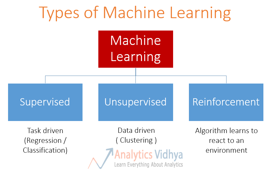
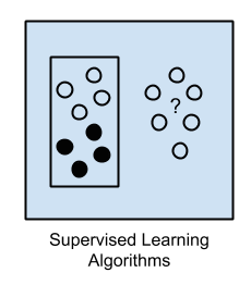
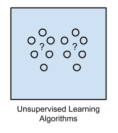
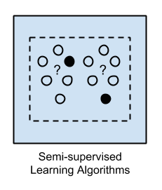
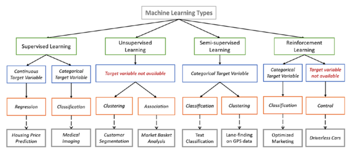

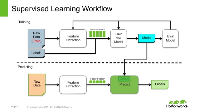
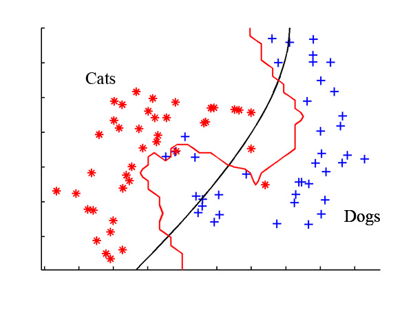
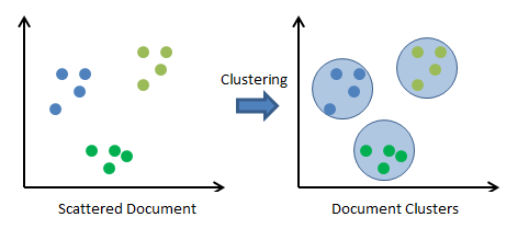


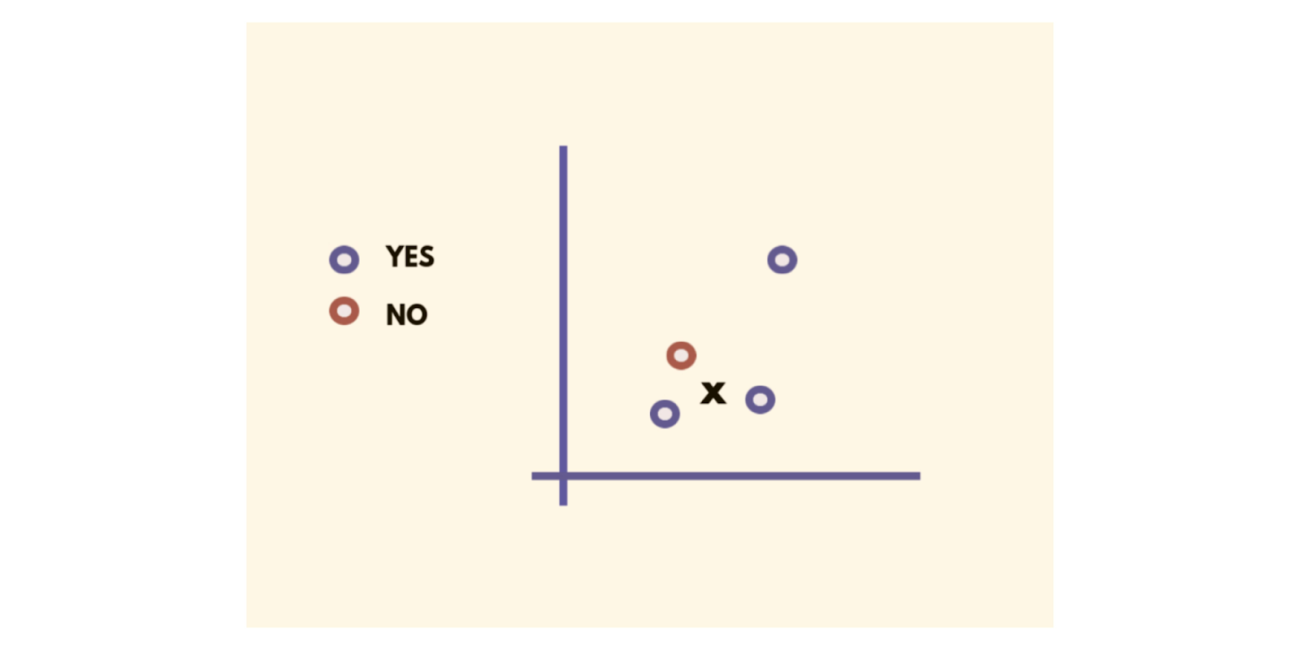
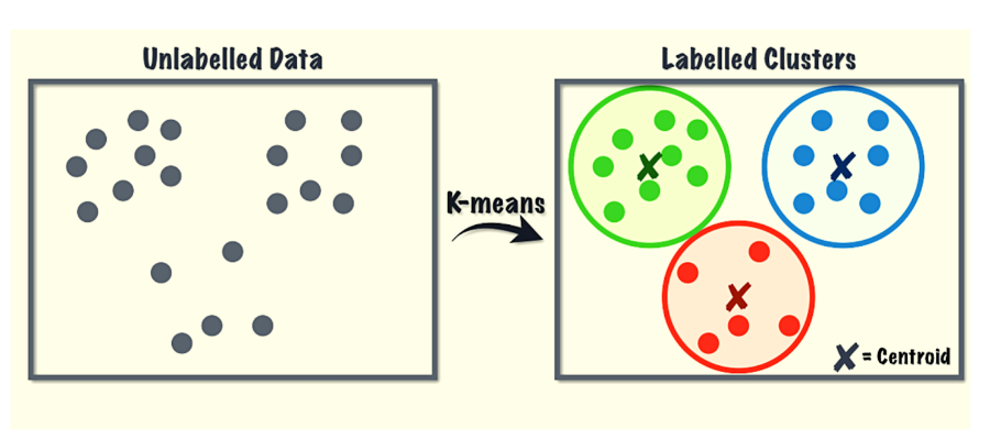

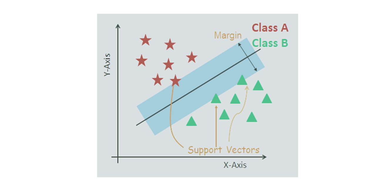


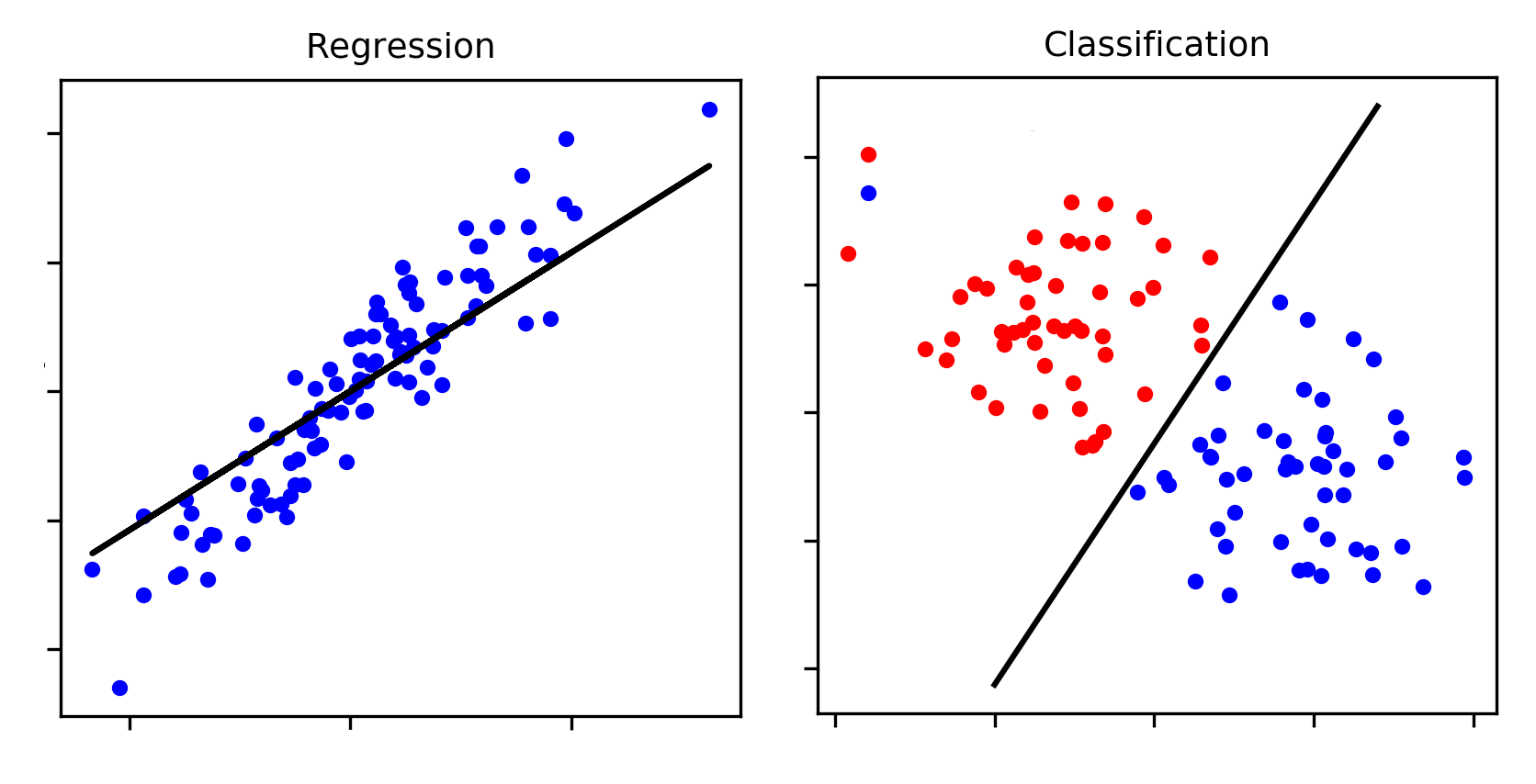
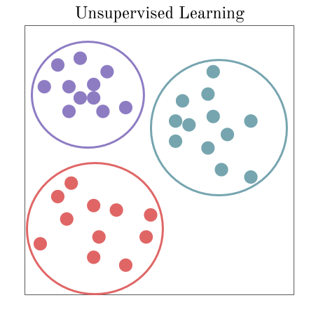
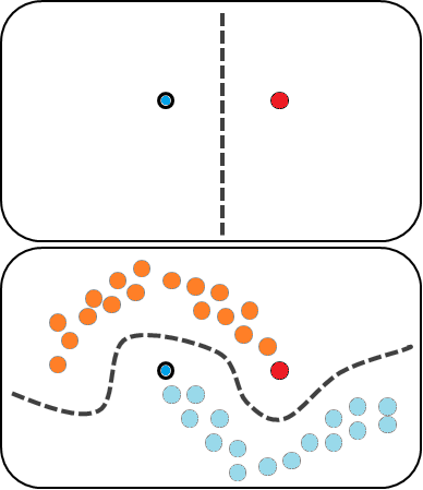

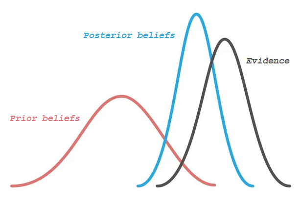
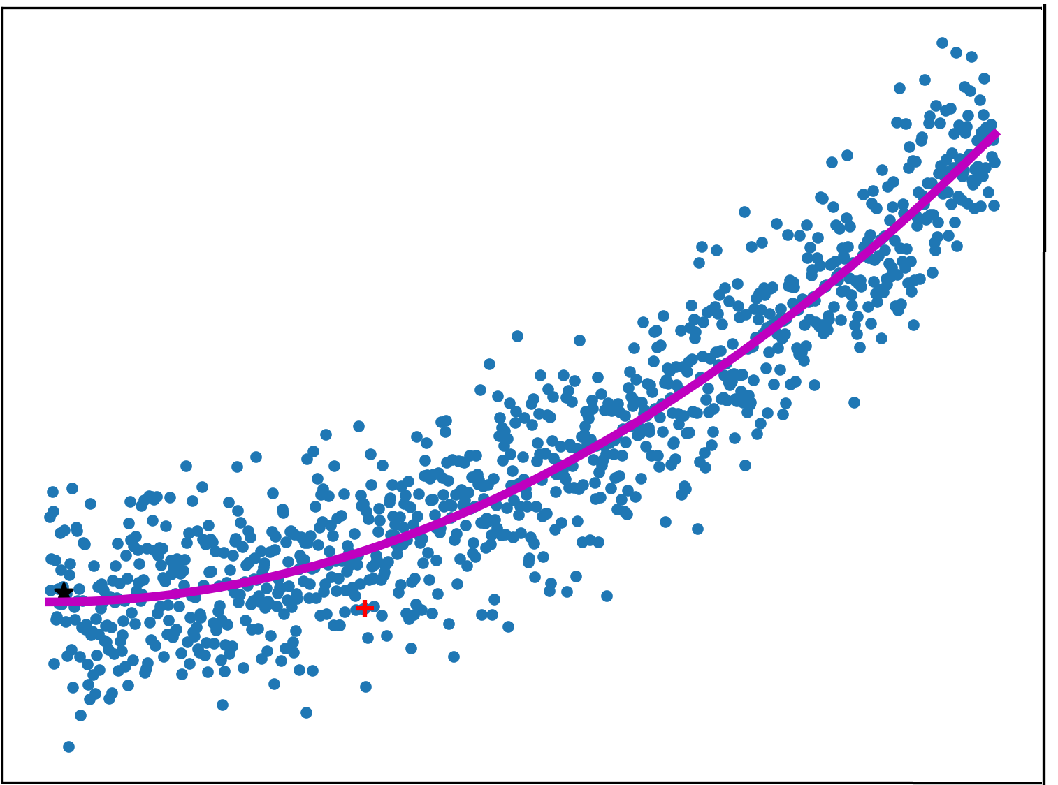

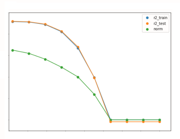
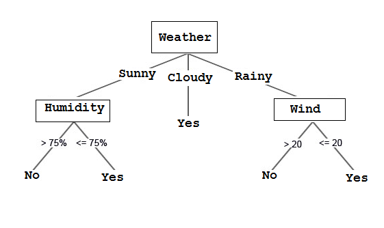
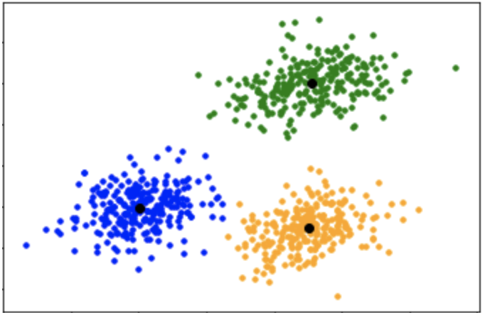
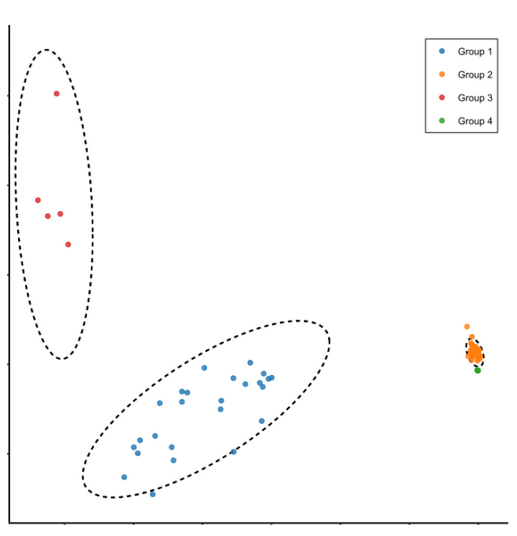
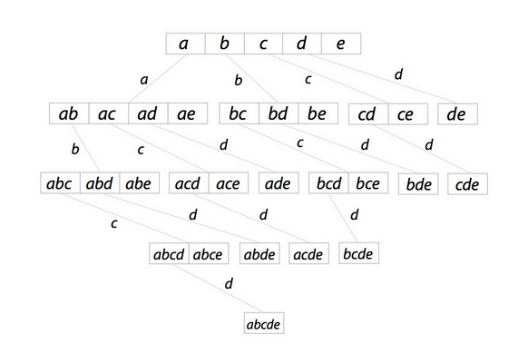
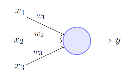
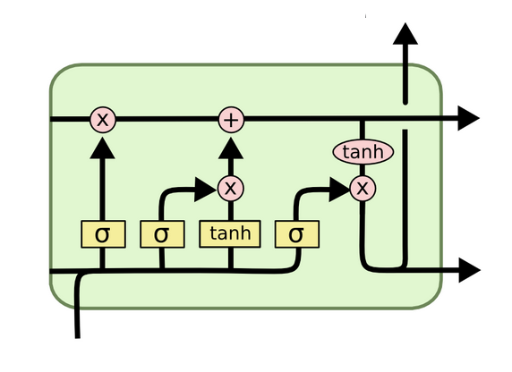
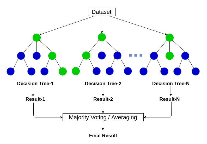
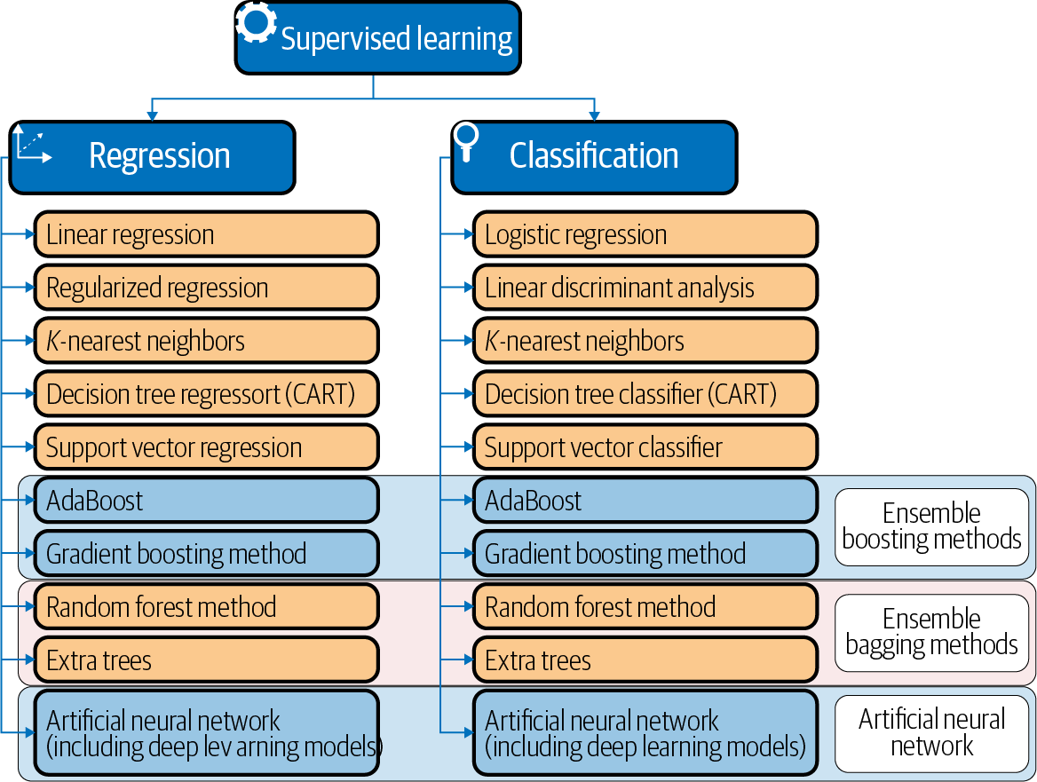
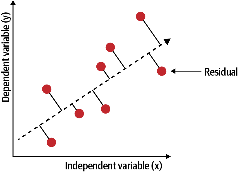
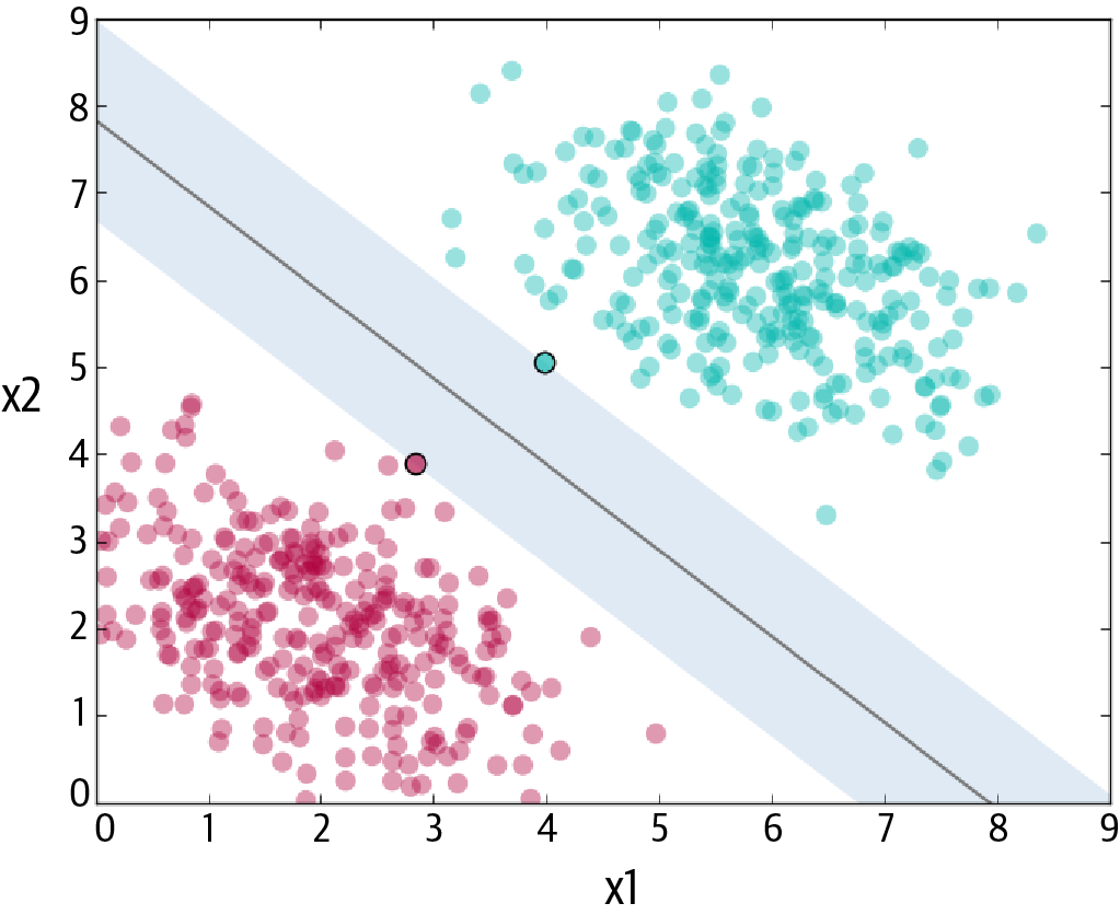
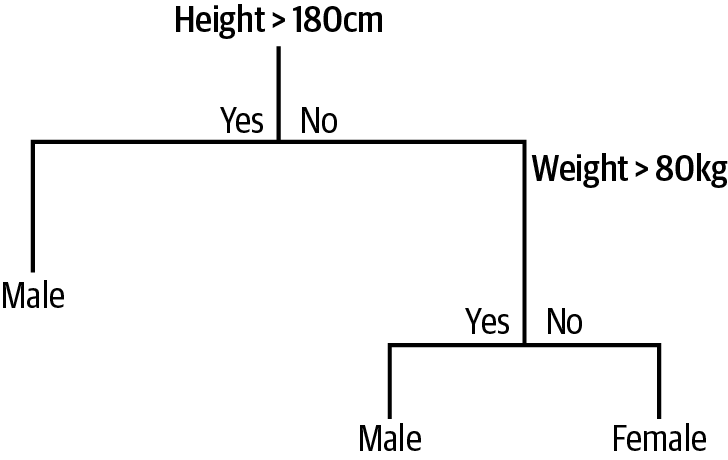
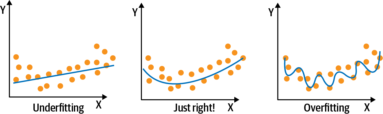
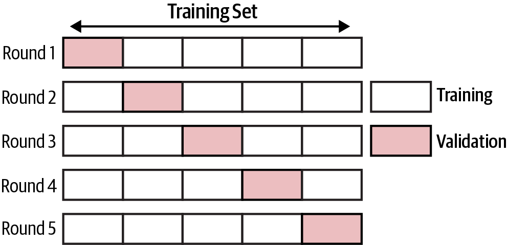
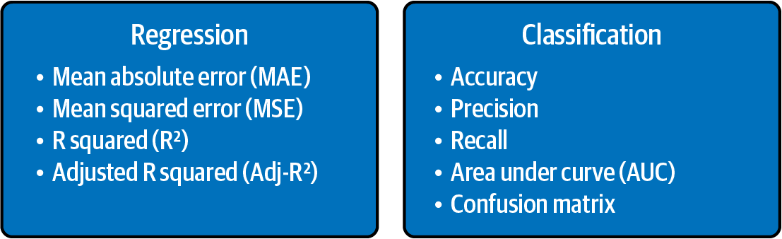
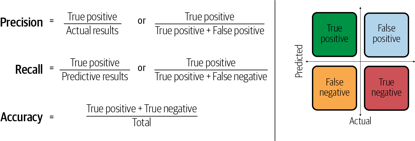
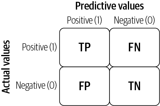
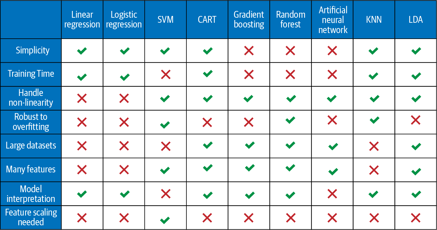

 Building intelligent robotics